


 MMUPHin是一个R包,用于微生物群落概况的荟萃分析,包括批次效应矫正、差异丰度检验和无监督聚类。本文介绍了如何使用MMUPHin进行数据处理,展示了在结直肠癌研究中校正批次效应和检测微生物差异的方法。
使用MMUPHin进行微生物组研究的荟萃分析
参考:
- 教程: https://bioconductor.org/packages/release/bioc/vignettes/MMUPHin/inst/doc/MMUPHin.html
- 参考文献: Ma S, Shungin D, Mallick H, et al. Population structure discovery in meta-analyzed microbial communities and inflammatory bowel disease using MMUPHin[J]. Genome Biology, 2022, 23(1): 1-31.
文章目录
1. 引言(Introduction)
MMUPHin是一个用于实现微生物群落概况的荟萃分析方法的R包。它具有以下接口:a)协变量控制的批处理和批次效应矫正,b)荟萃分析差异丰度检验,以及c)离散(基于聚类)或d)连续无监督种群结构的荟萃分析发现。
总体而言,MMUPHin能够实现多个微生物群落研究的标准化和组合。然后,它可以帮助识别在组合表型方面存在差异的微生物、基因或途径。最后,它可以找到在研究中一致再现的样本类型的聚类或梯度。
2. 安装(Installation)
MMUPHin是一个Bioconductor包,可以通过以下命令进行安装。
if (!requireNamespace("BiocManager", quietly = TRUE))
    install.packages("BiocManager")
BiocManager::install("MMUPHin")
本教程旨在为MMUPHin的所有四个功能提供工作示例。
MMUPHin可以通过下面显示的第一个library()命令加载到R中。我们还加载了一些用于数据操作和可视化的实用程序包。
library(MMUPHin)
library(magrittr)
library(dplyr)
library(ggplot2)
3. 输入数据(Input data)
作为输入,MMUPHin需要一个适当格式的微生物群落研究集合,包括特征丰度和附带的元数据。在这里,我们使用了Thomas等人(2019年)发表的五项结直肠癌(CRC)大便宏基因组研究。研究数据已经通过Biocondcutor软件curatedMetagenomicData方便地打包和访问,尽管还需要额外的步骤来格式化MMUPHin的输入。
重要的是,MMUPHin要求将特征丰度作为特征样本矩阵(feature-by-sample matrix)提供,并将元数据作为数据帧提供。这两个对象必须在样本ID上一致,即特征丰度矩阵的colname和元数据数据帧的rowname必须一致。R中许多流行的组学数据类已经强制执行了这一标准,例如Biobase的ExpressionSet或phyloseq的phyloseq。
为了最大限度地减少用户加载数据以运行示例的工作量,我们对五项研究进行了适当的格式化,以便于访问。特征的丰富程度和元数据可以用下面的代码块加载。对于感兴趣的用户,注释掉的脚本用于直接从curatedMetagenomicData访问数据并进行格式化。通读这些可能是值得的,因为它们执行许多预处理R中微生物特征丰度数据的常见任务,包括样本/特征子集设置(sample/feature subsetting)、归一化(normalization)、过滤(filtering)等。
data("CRC_abd", "CRC_meta")  ##加载数据
CRC_abd[1:5, 1, drop = FALSE] ##检查特征样本矩阵。
输出为:
##                                 FengQ_2015.metaphlan_bugs_list.stool:SID31004
## s__Faecalibacterium_prausnitzii                                    0.11110668
## s__Streptococcus_salivarius                                        0.09660736
## s__Ruminococcus_sp_5_1_39BFAA                                      0.09115385
## s__Subdoligranulum_unclassified                                    0.05806767
## s__Bacteroides_stercoris                                           0.05685503
CRC_meta[1, 1:5]
输出为:
##                                               subjectID body_site
## FengQ_2015.metaphlan_bugs_list.stool:SID31004  SID31004     stool
##                                               study_condition
## FengQ_2015.metaphlan_bugs_list.stool:SID31004             CRC
##                                                                    disease
## FengQ_2015.metaphlan_bugs_list.stool:SID31004 CRC;fatty_liver;hypertension
##                                               age_category
## FengQ_2015.metaphlan_bugs_list.stool:SID31004        adult
table(CRC_meta$studyID)
输出为:
##
##      FengQ_2015.metaphlan_bugs_list.stool
##                                       107
## HanniganGD_2017.metaphlan_bugs_list.stool
##                                        55
##  VogtmannE_2016.metaphlan_bugs_list.stool
##                                       104
##        YuJ_2015.metaphlan_bugs_list.stool
##                                       128
##    ZellerG_2014.metaphlan_bugs_list.stool
##                                       157
4. 使用adjust_batch进行批次矫正分析
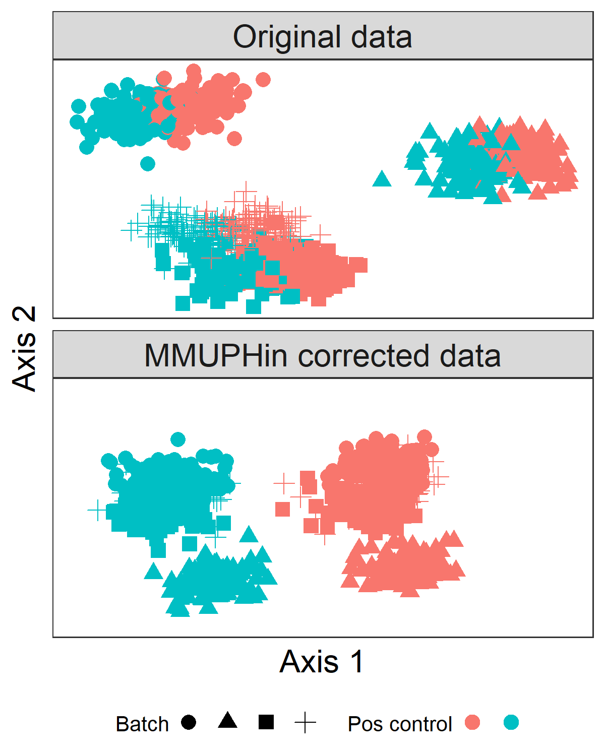
adjust_batch旨在纠正微生物特征丰度的技术研究/批次效应。它以样本丰度矩阵(feature-by-sample abundance matrix)的特征作为输入,并在给定的批次和可选协变量的情况下进行批次效应调整。它返回批量调整后的丰度矩阵。查看help(adjust_batch)以了解更多详细信息和选项。这张来自论文的图(图2b)显示了批次矫正的预期效果:批量效应被去除,使感兴趣的生物变量的影响更容易检测。
在这里,我们使用adjust_batch来校正五项研究中的差异,同时控制CRC与对照的影响(CRC_meta中的变量study_condition)。
adjust_batch返回多个输出的列表。我们现在最感兴趣的部分是调整后的丰度表,我们将其分配给CRC_abd_aj。
##Zero-inflated empirical Bayes adjustment of batch effect in compositional feature abundance data
fit_adjust_batch <- adjust_batch(feature_abd = CRC_abd,
                                 batch = "studyID",
                                 covariates = "study_condition",
                                 data = CRC_meta,
                                 control = list(verbose = FALSE))

CRC_abd_adj <- fit_adjust_batch$feature_abd_adj
评估批量调整效果的一种方法是评估调整前后可归因于研究差异的微生物谱的总变异性。这通常被称为PERMANOVA检验(Tang,Chen,and Alekseyenko 2016),可以使用vegan中的adonis函数进行。adonis的输入是微生物组成差异的指标。
##加载vegan包
library(vegan, quietly = TRUE)
输出为:
## This is vegan 2.6-4
##Dissimilarity Indices for Community Ecologists
D_before <- vegdist(t(CRC_abd))  ##默认计算Bray–Curtis距离。
D_after <- vegdist(t(CRC_abd_adj))

##Permutational Multivariate Analysis of Variance Using Distance Matrices
##置换多元回归方差分析。
set.seed(1)
fit_adonis_before <- adonis(D_before ~ studyID, data = CRC_meta)
输出为:
## 'adonis' will be deprecated: use 'adonis2' instead
##打印批次矫正前的置换多元回归方差分析的结果。
print(fit_adonis_before$aov.tab)
输出为:
## Permutation: free
## Number of permutations: 999
##
## Terms added sequentially (first to last)
##
##            Df SumsOfSqs MeanSqs F.Model      R2 Pr(>F)
## studyID     4     13.36  3.3400  11.855 0.07991  0.001 ***
## Residuals 546    153.82  0.2817         0.92009
## Total     550    167.18                 1.00000
## ---
## Signif. codes:  0 '***' 0.001 '**' 0.01 '*' 0.05 '.' 0.1 ' ' 1
##打印批次矫正后的置换多元回归方差分析的结果。
print(fit_adonis_after$aov.tab)
输出为:
## Permutation: free
## Number of permutations: 999
##
## Terms added sequentially (first to last)
##
##            Df SumsOfSqs MeanSqs F.Model      R2 Pr(>F)
## studyID     4     4.939 1.23463  4.2855 0.03044  0.001 ***
## Residuals 546   157.298 0.28809         0.96956
## Total     550   162.237                 1.00000
## ---
## Signif. codes:  0 '***' 0.001 '**' 0.01 '*' 0.05 '.' 0.1 ' ' 1
我们可以看到,在研究批次矫正之前,研究差异可解释微生物丰度谱差异的7.99%,而在调整之后,可解释的差异比例减少到3.04%,尽管研究的效应在这两种情况下都是显著的。
5. 使用lm_meta进行荟萃分析差异丰度检验
最常见的荟萃分析目标之一是将各批次/研究的关联效应相结合,以确定一致的总体效果。lm_meta为这项任务提供了一个简单的界面,首先使用经过充分验证的Maaslin2软件包在单个批次/研究中进行回归分析,然后通过vegan软件包将结果与已建立的固定/混合效应模型进行汇总。在这里,我们使用lm_meta来测试五项研究中CRC和对照样本之间一致差异丰富的物种,同时控制人口统计学协变量(gender、age、BMI)。同样,lm_meta返回一个包含多个组件的列表。meta_fits提供最终的荟萃分析检验结果。有关其他组件的含义,请参阅help(lm_meta)。
##Covariate adjusted meta-analytical differential abundance testing
fit_lm_meta <- lm_meta(feature_abd = CRC_abd_adj,
                       batch = "studyID",
                       exposure = "study_condition",
                       covariates = c("gender", "age", "BMI"),
                       data = CRC_meta,
                       control = list(verbose = FALSE))
输出为:
## Warning in lm_meta(feature_abd = CRC_abd_adj, batch = "studyID", exposure = "study_condition", : Covariate gender is missing or has only one non-missing value in the following batches; will be excluded from model for these batches:
## HanniganGD_2017.metaphlan_bugs_list.stool, YuJ_2015.metaphlan_bugs_list.stool
## Warning in lm_meta(feature_abd = CRC_abd_adj, batch = "studyID", exposure = "study_condition", : Covariate age is missing or has only one non-missing value in the following batches; will be excluded from model for these batches:
## HanniganGD_2017.metaphlan_bugs_list.stool, YuJ_2015.metaphlan_bugs_list.stool
## Warning in lm_meta(feature_abd = CRC_abd_adj, batch = "studyID", exposure = "study_condition", : Covariate BMI is missing or has only one non-missing value in the following batches; will be excluded from model for these batches:
## HanniganGD_2017.metaphlan_bugs_list.stool, YuJ_2015.metaphlan_bugs_list.stool
结果为:
meta_fits <- fit_lm_meta$meta_fits
您会注意到,这个命令会产生一些错误消息。这是因为其中一项研究没有测量特定的协变量。正如消息所述,在分析该研究的数据时,这些协变量不包括在内。我们还注意到,批量校正是标准的,但对于这里的分析来说不是必要的。
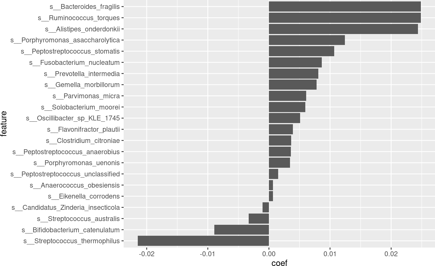
我们可以在这些研究/样本中看到与CRC相关的显著物种(FDR q<0.05)。将它们与Thomas等人(2019)的图1b进行比较,我们可以看到许多重要物种确实达成了一致。
meta_fits %>%
  filter(qval.fdr < 0.05) %>%
  arrange(coef) %>%
  mutate(feature = factor(feature, levels = feature)) %>%
  ggplot(aes(y = coef, x = feature)) +
  geom_bar(stat = "identity") +
  coord_flip()
6. 使用discrete_discover识别离散群落结果
微生物图谱的聚类分析有助于识别有意义的离散种群亚群(Ravel等人,2011),但必须仔细进行验证,以确保识别的结构是一致的(Koren等人,2013)。discrete_discover提供了使用预测强度(Tibshirani和Walther 2005)来评估单个微生物研究中的离散聚类结构的功能,以及评估其在其他研究中的再现性的“广义预测强度”。这些共同提供了荟萃分析的证据,用于(或反对)鉴定微生物图谱中的离散种群结构。查看help(discite_discover)以查看有关该方法和其他选项的更多详细信息。我们可以将离散结构(集群)与连续结构(将在下一节中进行概述)进行对比:
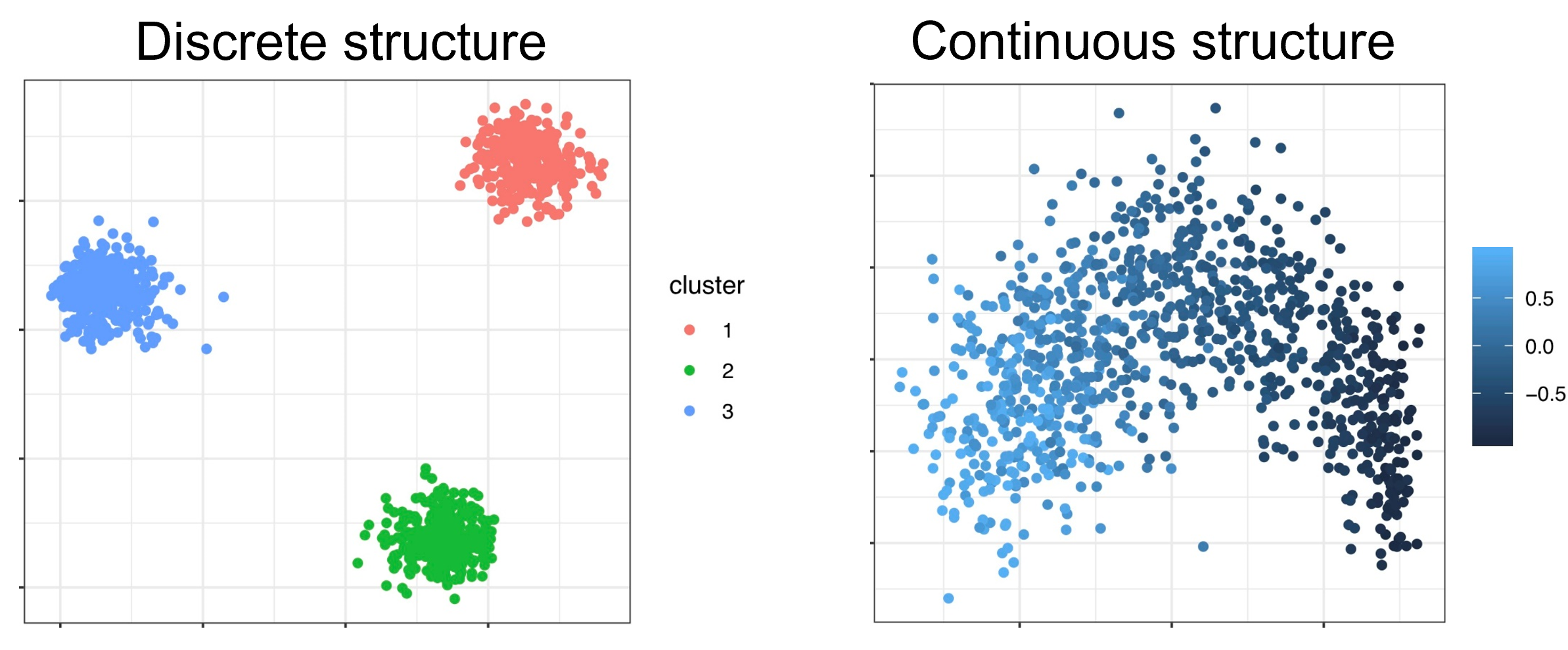
众所周知,肠道微生物组会形成梯度,而不是离散的集群(Koren等人,2013)。在这里,我们使用discrete_discover来评估五项粪便研究中对照样本之间的聚类结构。值得注意的是,该函数以距离/差异度矩阵作为输入,而不是丰度表。
control_meta <- subset(CRC_meta, study_condition == "control")
control_abd_adj <- CRC_abd_adj[, rownames(control_meta)]

D_control <- vegdist(t(control_abd_adj))

##Unsupervised meta-analytical discovery and validation of discrete clustering structures in microbial abundance data
fit_discrete <- discrete_discover(D = D_control,
                                  batch = "studyID",
                                  data = control_meta,
                                  control = list(k_max = 8,
                                                 verbose = FALSE))
fit_displete的internal_mean和internal_sd分量是提供每个批次(列)的内部评估统计信息(预测强度)和评估的聚类数量(行)的矩阵。类似地,external_mean和external_sd提供外部评估统计数据(广义预测强度)。离散结构存在的证据将是在特定簇数处平均统计的“峰值”。在这里,为了更容易地检查这种模式,我们可视化了最大的研究ZellerG_2014的结果。请注意,默认情况下,所有研究的可视化都会自动生成并保存到输出文件“diagnostic_discrete.pdf”中。
study_id = "ZellerG_2014.metaphlan_bugs_list.stool"

internal <- data.frame(K = 2:8,
                       statistic = fit_discrete$internal_mean[, study_id],
                       se = fit_discrete$internal_se[, study_id],
                       type = "internal")

external <- data.frame(K = 2:8,
                       statistic = fit_discrete$external_mean[, study_id],
                       se = fit_discrete$external_se[, study_id],
                       type = "external")

rbind(internal, external) %>%
  ggplot(aes(x = K, y = statistic, color = type)) +
  geom_point(position = position_dodge(width = 0.5)) +
  geom_line(position = position_dodge(width = 0.5)) +
  geom_errorbar(aes(ymin = statistic - se, ymax = statistic + se),
                position = position_dodge(width = 0.5), width = 0.5) +
  ggtitle("Evaluation of discrete structure in control stool microbiome (ZellerG_2014)")
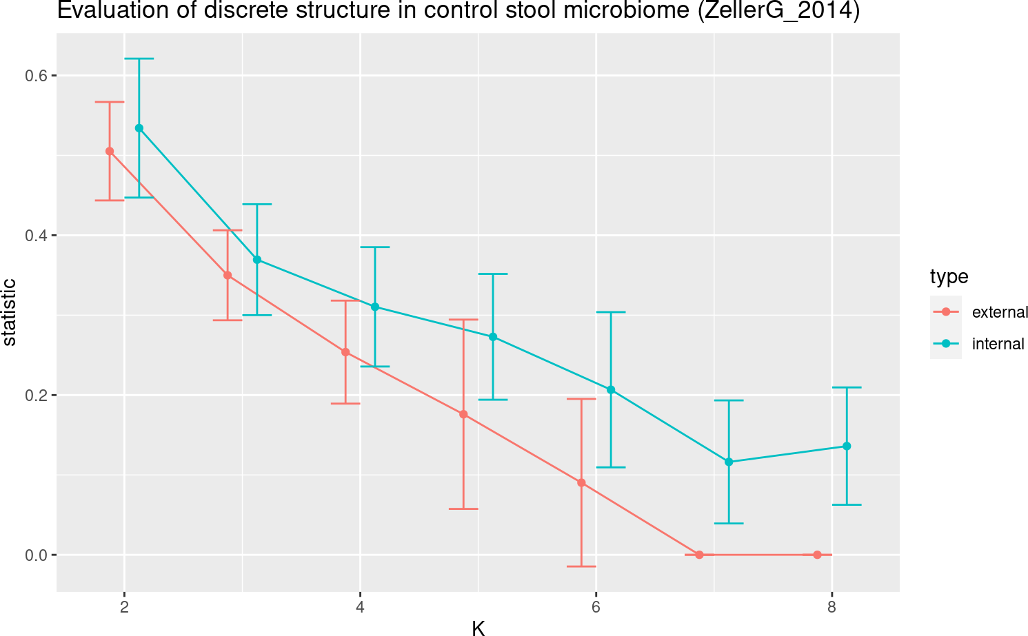
内部和外部统计数据以及集群数量(K)的下降趋势表明,离散结构无法建立。为了提供一个积极的例子,我们检查了由curatedMetagenomicData提供的两项阴道微生物组研究,因为已知阴道微生物组具有不同的亚型(Ravel等人,2011)。同样,我们预先格式化了这些数据集,以便于访问,但您可以使用注释掉的脚本从curatedMetagenomicData中重新创建它们。
data("vaginal_abd", "vaginal_meta")
D_vaginal <- vegdist(t(vaginal_abd))

fit_discrete_vag <- discrete_discover(D = D_vaginal,
                                      batch = "studyID",
                                      data = vaginal_meta,
                                      control = list(verbose = FALSE,
                                                     k_max = 8))

hmp_id = "HMP_2012.metaphlan_bugs_list.vagina"
data.frame(K = 2:8,
           statistic = fit_discrete_vag$internal_mean[, hmp_id],
           se = fit_discrete_vag$internal_se[, hmp_id]) %>%
  ggplot(aes(x = K, y = statistic)) +
  geom_point() +
  geom_line() +
  geom_errorbar(aes(ymin = statistic - se,
                    ymax = statistic + se),
                width = 0.5) +
  ggtitle("Evaluation of discrete structure in vaginal microbiome (HMP_2012)")
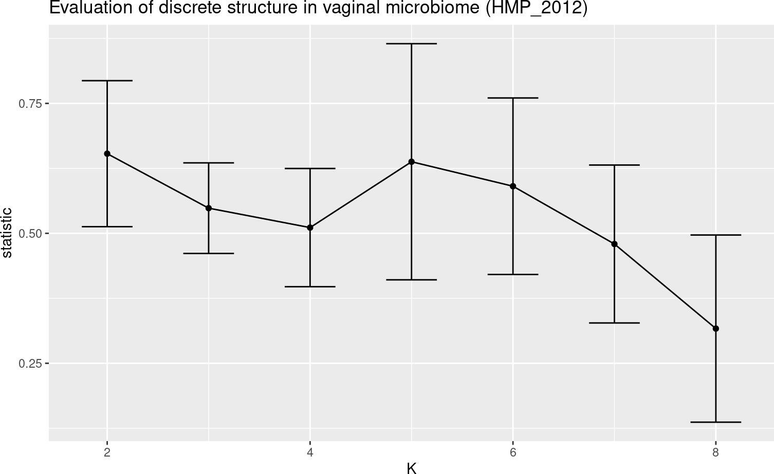
我们可以看到,对于阴道微生物组,discret_discover表明存在五个集群。在这里,我们只检查HMP_2012的内部指标,因为另一项研究(FerrettiP_2018)只有19个样本。
7. 使用continuous_discover识别连续群落结构
微生物组中的种群结构可以表现为梯度,而不是离散的集群,例如优势门权衡或疾病相关的微生态失调。continuous_discover提供了识别此类结构以及通过荟萃分析验证这些结构的功能。我们在五项研究的对照样本中再次评估这些连续结构。
与adjust_batch和lm_meta非常相似,continuous_discover也以样本丰度作为输入特征。控制参数提供了许多调整参数,这里我们将其中一个参数var_perc_cutoff设置为0.5,这要求该方法在每个批次中包括顶部主成分,这些成分总共解释了批次中至少50%的总可变性。有关调整参数及其解释的更多详细信息,请参阅help(continuous_discover)。
fit_continuous <- continuous_discover(feature_abd = control_abd_adj,
                                      batch = "studyID",
                                      data = control_meta,
                                      control = list(var_perc_cutoff = 0.5,
                                                     verbose = FALSE))
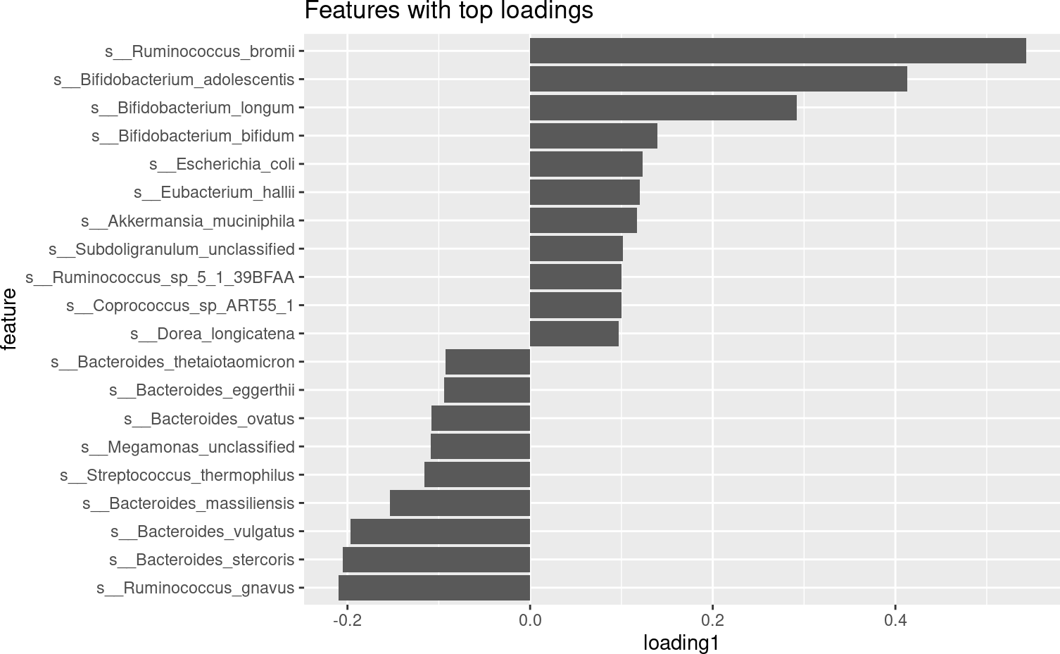
我们可以通过至少两种方式可视化已识别的连续结构分数:首先,检查其最重要的微生物特征,了解分数的特征,其次,用坐标可视化(an ordination visualization)覆盖连续分数。在这里,我们对第一个确定的连续分数进行这些可视化。
loading <- data.frame(feature = rownames(fit_continuous$consensus_loadings),
                      loading1 = fit_continuous$consensus_loadings[, 1])

loading %>%
    arrange(-abs(loading1)) %>%
    slice(1:20) %>%
    arrange(loading1) %>%
    mutate(feature = factor(feature, levels = feature)) %>%
    ggplot(aes(x = feature, y = loading1)) +
    geom_bar(stat = "identity") +
    coord_flip() +
    ggtitle("Features with top loadings")
mds <- cmdscale(d = D_control)
colnames(mds) <- c("Axis1", "Axis2")
as.data.frame(mds) %>%
  mutate(score1 = fit_continuous$consensus_scores[, 1]) %>%
  ggplot(aes(x = Axis1, y = Axis2, color = score1)) +
  geom_point() +
  coord_fixed()
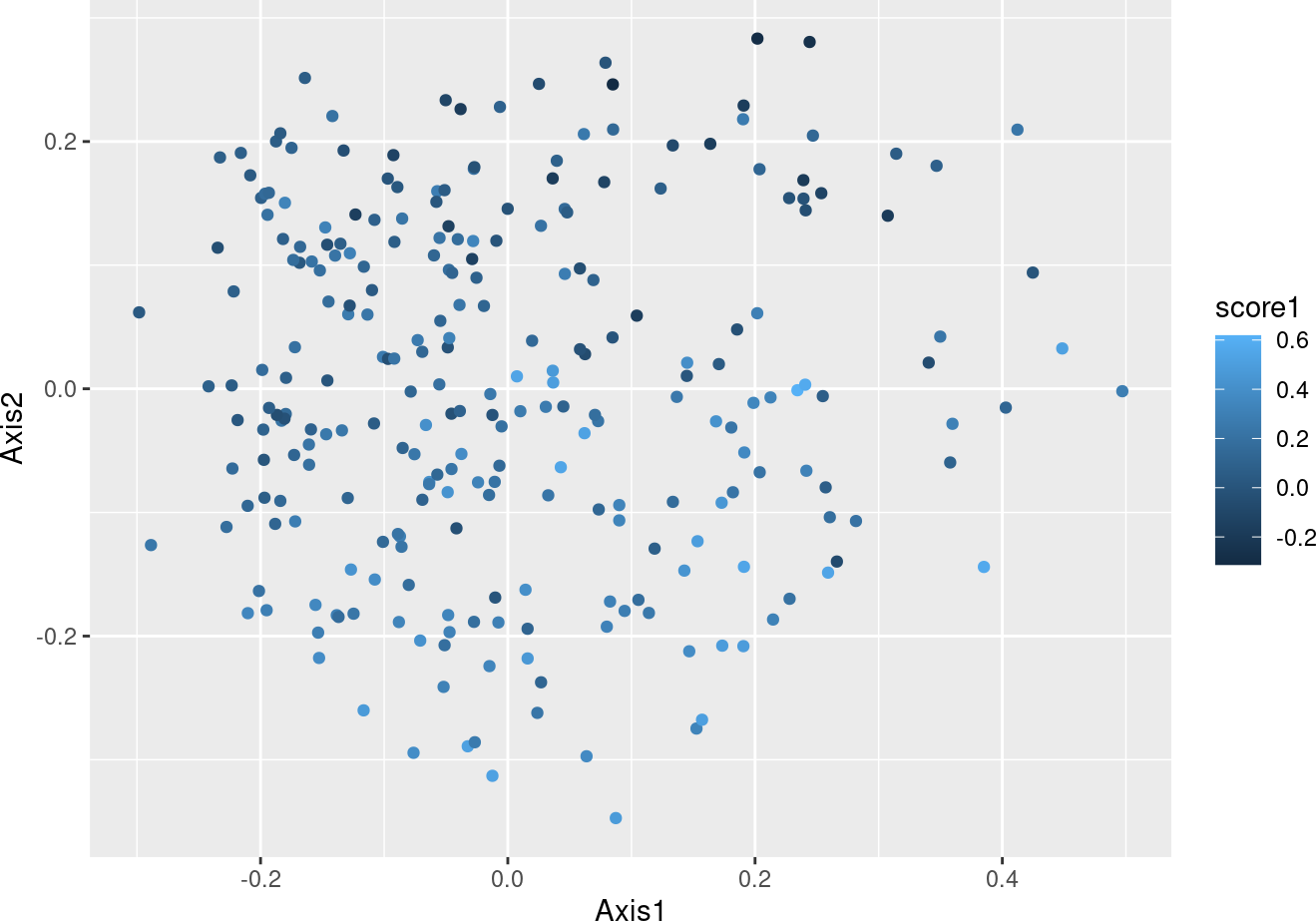
从排序中我们可以看出,第一个连续评分确实代表了这些粪便样本之间的强烈差异。从最高负荷特征中,我们可以看到,这一分数强烈代表了拟杆菌门(Bacteroides属物种)与厚壁菌门(Ruminococcus 属物种)的权衡。
8. Sessioninfo
sessionInfo() ##检查sessionInfo。
## R version 4.3.0 RC (2023-04-13 r84269)
## Platform: x86_64-pc-linux-gnu (64-bit)
## Running under: Ubuntu 22.04.2 LTS
##
## Matrix products: default
## BLAS:   /home/biocbuild/bbs-3.17-bioc/R/lib/libRblas.so
## LAPACK: /usr/lib/x86_64-linux-gnu/lapack/liblapack.so.3.10.0
##
## locale:
##  [1] LC_CTYPE=en_US.UTF-8       LC_NUMERIC=C
##  [3] LC_TIME=en_GB              LC_COLLATE=C
##  [5] LC_MONETARY=en_US.UTF-8    LC_MESSAGES=en_US.UTF-8
##  [7] LC_PAPER=en_US.UTF-8       LC_NAME=C
##  [9] LC_ADDRESS=C               LC_TELEPHONE=C
## [11] LC_MEASUREMENT=en_US.UTF-8 LC_IDENTIFICATION=C
##
## time zone: America/New_York
## tzcode source: system (glibc)
##
## attached base packages:
## [1] stats     graphics  grDevices utils     datasets  methods   base
##
## other attached packages:
## [1] vegan_2.6-4      lattice_0.21-8   permute_0.9-7    ggplot2_3.4.2
## [5] dplyr_1.1.2      magrittr_2.0.3   MMUPHin_1.14.0   BiocStyle_2.28.0
##
## loaded via a namespace (and not attached):
##  [1] tidyselect_1.2.0    farver_2.1.1        fastmap_1.1.1
##  [4] mathjaxr_1.6-0      digest_0.6.31       lifecycle_1.0.3
##  [7] cluster_2.1.4       kernlab_0.9-32      compiler_4.3.0
## [10] rlang_1.1.0         sass_0.4.5          tools_4.3.0
## [13] igraph_1.4.2        utf8_1.2.3          yaml_2.3.7
## [16] knitr_1.42          labeling_0.4.2      mclust_6.0.0
## [19] withr_2.5.0         purrr_1.0.1         numDeriv_2016.8-1.1
## [22] nnet_7.3-18         grid_4.3.0          pcaPP_2.0-3
## [25] hash_2.2.6.2        stats4_4.3.0        fansi_1.0.4
## [28] Maaslin2_1.14.0     colorspace_2.1-0    scales_1.2.1
## [31] fpc_2.2-10          MASS_7.3-59         prabclus_2.3-2
## [34] logging_0.10-108    optparse_1.7.3      cli_3.6.1
## [37] mvtnorm_1.1-3       rmarkdown_2.21      metafor_4.0-0
## [40] crayon_1.5.2        ragg_1.2.5          generics_0.1.3
## [43] robustbase_0.95-1   biglm_0.9-2.1       getopt_1.20.3
## [46] DBI_1.1.3           pbapply_1.7-0       cachem_1.0.7
## [49] stringr_1.5.0       modeltools_0.2-23   splines_4.3.0
## [52] metadat_1.2-0       parallel_4.3.0      BiocManager_1.30.20
## [55] vctrs_0.6.2         Matrix_1.5-4        jsonlite_1.8.4
## [58] bookdown_0.33       systemfonts_1.0.4   magick_2.7.4
## [61] diptest_0.76-0      tidyr_1.3.0         jquerylib_0.1.4
## [64] glue_1.6.2          DEoptimR_1.0-12     cowplot_1.1.1
## [67] stringi_1.7.12      gtable_0.3.3        munsell_0.5.0
## [70] lpsymphony_1.28.0   tibble_3.2.1        pillar_1.9.0
## [73] htmltools_0.5.5     R6_2.5.1            textshaping_0.3.6
## [76] evaluate_0.20       highr_0.10          bslib_0.4.2
## [79] class_7.3-21        Rcpp_1.0.10         flexmix_2.3-19
## [82] nlme_3.1-162        mgcv_1.8-42         xfun_0.39
## [85] pkgconfig_2.0.3
参考文献(References)
Koren, Omry, Dan Knights, Antonio Gonzalez, Levi Waldron, Nicola Segata, Rob Knight, Curtis Huttenhower, and Ruth E Ley. 2013. “A Guide to Enterotypes Across the Human Body: Meta-Analysis of Microbial Community Structures in Human Microbiome Datasets.” PLoS Computational Biology 9 (1): e1002863.
Ravel, Jacques, Pawel Gajer, Zaid Abdo, G Maria Schneider, Sara SK Koenig, Stacey L McCulle, Shara Karlebach, et al. 2011. “Vaginal Microbiome of Reproductive-Age Women.” Proceedings of the National Academy of Sciences 108 (Supplement 1): 4680–7.
Tang, Zheng-Zheng, Guanhua Chen, and Alexander V Alekseyenko. 2016. “PERMANOVA-S: Association Test for Microbial Community Composition That Accommodates Confounders and Multiple Distances.” Bioinformatics 32 (17): 2618–25.
Thomas, Andrew Maltez, Paolo Manghi, Francesco Asnicar, Edoardo Pasolli, Federica Armanini, Moreno Zolfo, Francesco Beghini, et al. 2019. “Metagenomic Analysis of Colorectal Cancer Datasets Identifies Cross-Cohort Microbial Diagnostic Signatures and a Link with Choline Degradation.” Nature Medicine 25 (4): 667.
Tibshirani, Robert, and Guenther Walther. 2005. “Cluster Validation by Prediction Strength.” Journal of Computational and Graphical Statistics 14 (3): 511–28.


 1617
1617

 被折叠的 条评论
为什么被折叠?
被折叠的 条评论
为什么被折叠?
 到【灌水乐园】发言


