AANAP代码学习

最新推荐文章于 2024-08-08 07:27:33 发布

原创最新推荐文章于 2024-08-08 07:27:33 发布 · 5.4k 阅读

40 ·

CC 4.0 BY-SA版权

图像视频拼接专栏收录该内容

3 篇文章

订阅专栏

Code:YaqiLYU/AANAP
Paper:Adaptive As-Natural-As-Possible Image Stitching

1、加载并显示图片
加载两幅图片：img1、img2，把img2大小resize为img1大小。

%% Global options
% 0 - Bilinear interpolation, implementation by MATLAB锛宻lower but better-->双线性插值
% 1 - Nearest neighbor interpolation,implementation by C++, Faster but worse---->最邻近插值
fast_stitch = 1;    
img_n = 2;  % only support two image stitching
in_name = cell(img_n,1);
in_name{1} = 'images/case26/img04.JPG';
in_name{2} = 'images/case26/img05.JPG';
img_n = size(in_name, 1);

gamma = 0;
sigma = 12.5;

%% load and preprocessing
I = cell(img_n, 1);
for i = 1 : img_n
    I{i} = imread(in_name{i});
end

max_size = 1000 * 1000;
imgw = zeros(img_n, 1);
imgh = zeros(img_n, 1);

for i = 1 : img_n
    if numel(I{i}(:, :, 1)) > max_size
        I{i} = imresize(I{i}, sqrt(max_size / numel(I{i}(:, :, 1))));
    end

    imgw(i) = size(I{i}, 2);
    imgh(i) = size(I{i}, 1);
end

img1 = I{1};
img2 = I{2};
img2 = imresize(img2,size(img1,1)/size(img2,1));

figure(4),
imshow(img1,[]);
pause(0.3);
figure(5),
imshow(img2,[]);
pause(0.3);

2、变量初始化

%% User defined parameters for APAP
clear global;
global fitfn resfn degenfn psize numpar
fitfn = 'homography_fit';   %计算Global H
resfn = 'homography_res';
degenfn = 'homography_degen';
psize   = 4;
numpar  = 9;

M     = 500;
thr_g = 0.1;    %RANSAC threshold

if fast_stitch
    C1    = 100;    %C1，C2为分块大小
    C2    = 100;
else
    C1    = 200;
    C2    = 200;
end

3、SIFT特征检测与匹配

[ kp1,ds1 ] = vl_sift(single(rgb2gray(img1)),'PeakThresh', 0,'edgethresh',500);
[ kp2,ds2 ] = vl_sift(single(rgb2gray(img2)),'PeakThresh', 0,'edgethresh',500);
[match_idxs, scores] = vl_ubcmatch(ds1,ds2);
f1 = kp1(:,match_idxs(1,:));
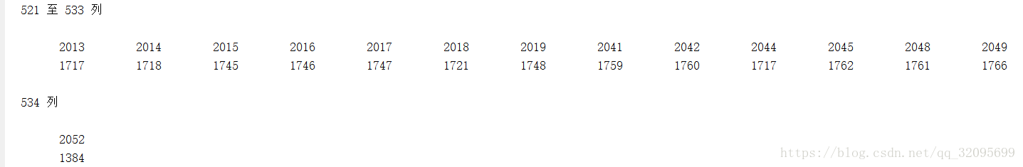
f2 = kp2(:,match_idxs(2,:));

kp1：img1的特征点(本例中kp1:4x2067，既找到了2067个特征点)
这里写图片描述

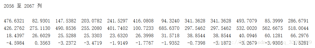
kp2：img2的特征点(本例中kp2：4x1779，既找到了1779个特征点)
这里写图片描述

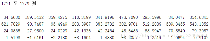
match_idxs:img1，img2匹配的特征点的索引：(本例中match_idxs：2x534，既找到了534个匹配对)
这里写图片描述

[F,D] = VL_SIFT(I)
F为特征点，D为描述子。

%   Each column of F is a feature frame and has the format [X;Y;S;TH], where 
%   X,Y is the (fractional) center of the frame, S is the scale and TH is
%   the orientation (in radians).

%   [F,D] = VL_SIFT(I) computes the SIFT descriptors [1] as well. Each
%   column of D is the descriptor of the corresponding frame in F. A
%   descriptor is a 128-dimensional vector of class UINT8.

4、匹配点归一化，用门限值 thr_g = 0.1 删除RANSAC的Outliner

%% Normalise point distribution and Outlier removal with Multi-GS RANSAC.
% (x1;y1;1;x2;y2;1)
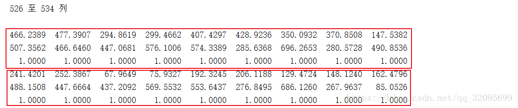
data_orig = [ kp1(1:2,match_idxs(1,:)) ; ones(1,size(match_idxs,2)) ;
              kp2(1:2,match_idxs(2,:)) ; ones(1,size(match_idxs,2)) ];
[ dat_norm_img1,T1 ] = normalise2dpts(data_orig(1:3,:));
[ dat_norm_img2,T2 ] = normalise2dpts(data_orig(4:6,:));
data_norm = [ dat_norm_img1 ; dat_norm_img2 ];

% Multi-GS
% rng(0);
[ ~,res,~,~ ] = multigsSampling(100,data_norm,M,10);
con = sum(res<=thr_g);
[ ~, maxinx ] = max(con);
inliers = find(res(:,maxinx)<=thr_g);%找到匹配度最高的特征点序列，inliers存的是匹配对的索引

data_orig：齐次坐标下所有匹配特征点的组合。(本例中data_orig：6x534，对应534个匹配对的坐标–>x1,y1,1;x2,y2,1)
这里写图片描述
[newpts, T] = normalise2dpts(pts):归一化函数
作用：把一系列的齐次坐标［x y 1］归一化，使得这些点以原点为中心，距离原点均值为sqrt(2)。


function [newpts, T] = normalise2dpts(pts)

    if size(pts,1) ~= 3
        error('pts must be 3xN');
    end

    % Find the indices of the points that are not at infinity
    finiteind = find(abs(pts(3,:)) > eps);%找出非无穷远点的序号

    if length(finiteind) ~= size(pts,2)
        disp('Some points are at infinity');
    end

    % For the finite points ensure homogeneous coords have scale of 1
    pts(1,finiteind) = pts(1,finiteind)./pts(3,finiteind);
    pts(2,finiteind) = pts(2,finiteind)./pts(3,finiteind);
    pts(3,finiteind) = 1;

    c = mean(pts(1:2,finiteind)')';            % Centroid of finite points （找出所有点的中值）
  % c =
  %368.3553
  %434.4607
    newp(1,finiteind) = pts(1,finiteind)-c(1); % Shift origin to centroid.
    newp(2,finiteind) = pts(2,finiteind)-c(2); % 其他特征点到中值点的偏移量

    dist = sqrt(newp(1,finiteind).^2 + newp(2,finiteind).^2);%其他特征点到中值点的距离
    meandist = mean(dist(:));  % Ensure dist is a column vector for Octave 3.0.1其他特征点到中值点的平均距离

    scale = sqrt(2)/meandist;

    T = [scale   0   -scale*c(1)
         0     scale -scale*c(2)
         0       0      1      ];

    newpts = T*pts;

end

T的作用相当于：
x’ = scale(x-c(1));
y’ = scale(y- c(2));

data_norm :归一化后的匹配点矩阵
这里写图片描述

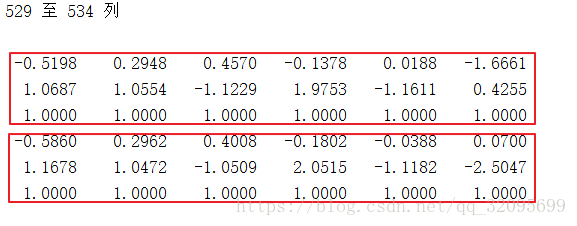
inliers:最佳匹配对索引：(本例中inliers：511x1，对应511个内点的索引)

RANSAC算法流程：
这里写图片描述
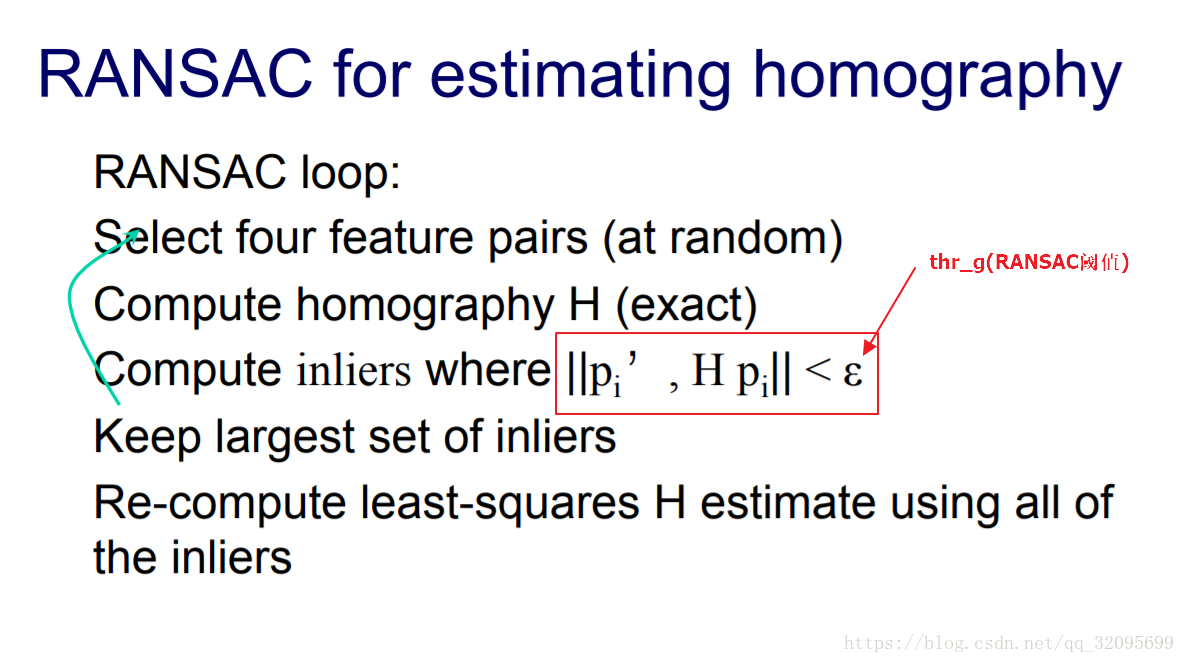
详情看slids:
Advances in Computer Vision
Lecture 9
Mid level vision:
Stereo, Homographies, RANSAC
5、通过内点计算Global H

%% Global homography (H) again.
[ Hl,A,D1,D2 ] = feval(fitfn,data_norm(:,inliers));
Hg = T2\(reshape(Hl,3,3)*T1);
Hg = Hg / Hg(3,3)

Hg =

1.3326    0.0151 -314.6591
0.2190    1.2556 -104.2045
0.0006    0.0000    1.0000

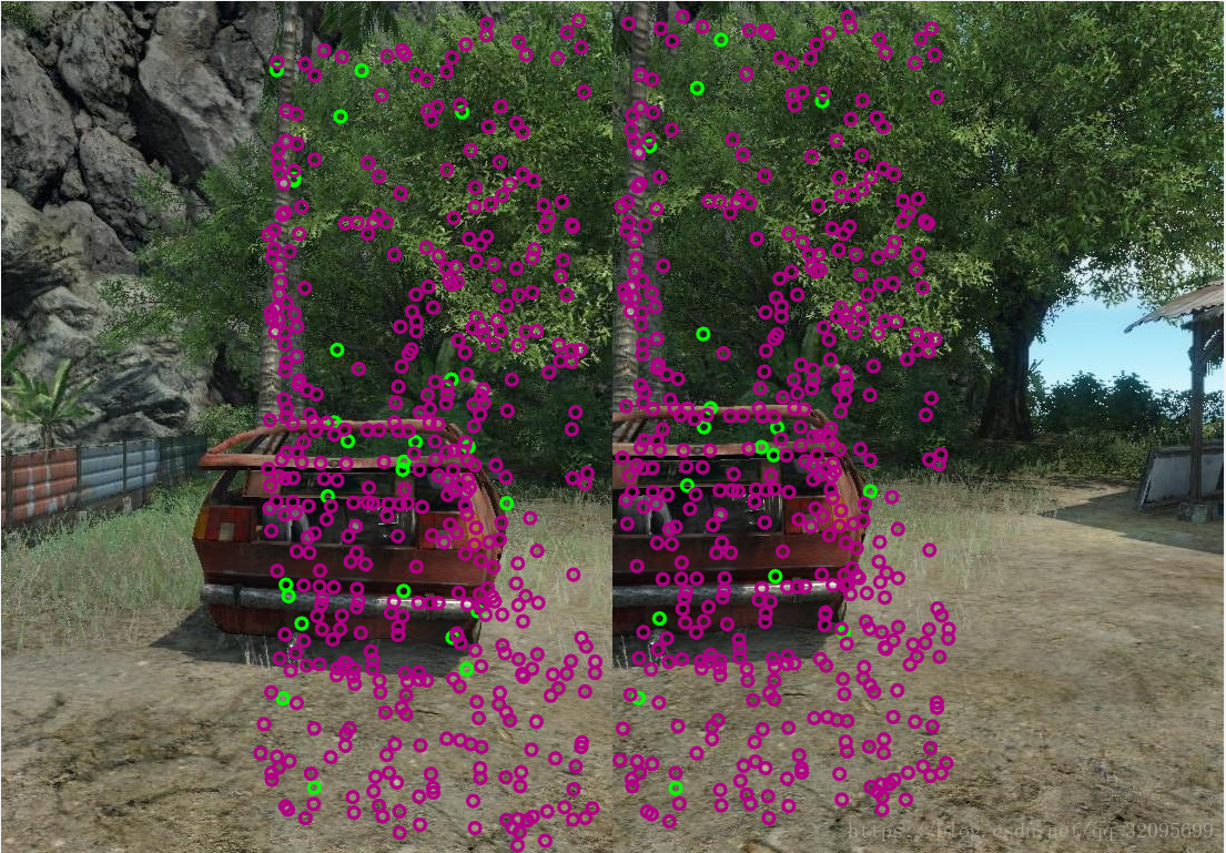
6、求Global similarity transformation—->S

%% Compute Global similarity
S = ransac_global_similarity(data_norm(:,inliers),data_orig(:,inliers),img1,img2);
S = T2\(S*T1)

先看看相似变换：图像的等距变换，相似变换，仿射变换，射影变换及其matlab实现
这里写图片描述
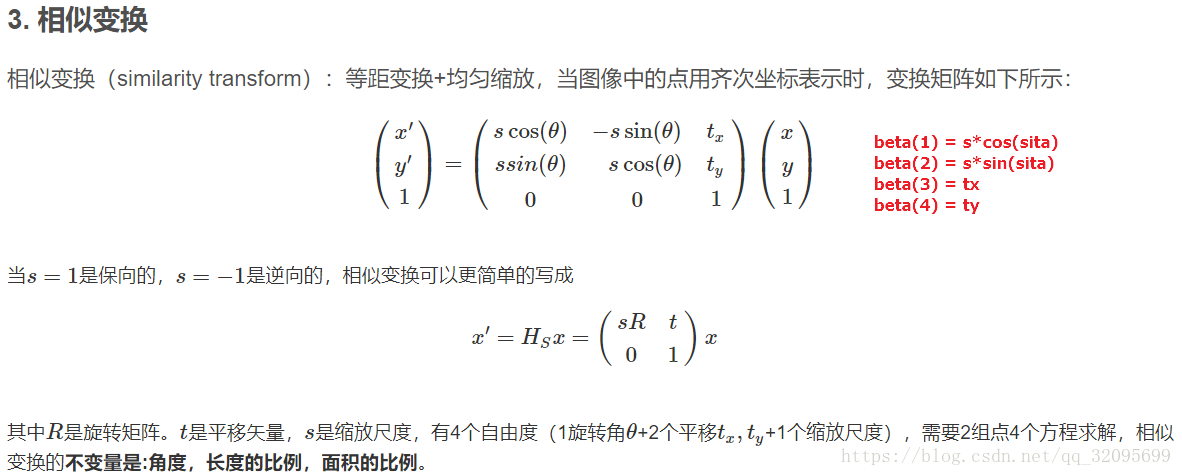
上述变换可以转换为：

对应代码：

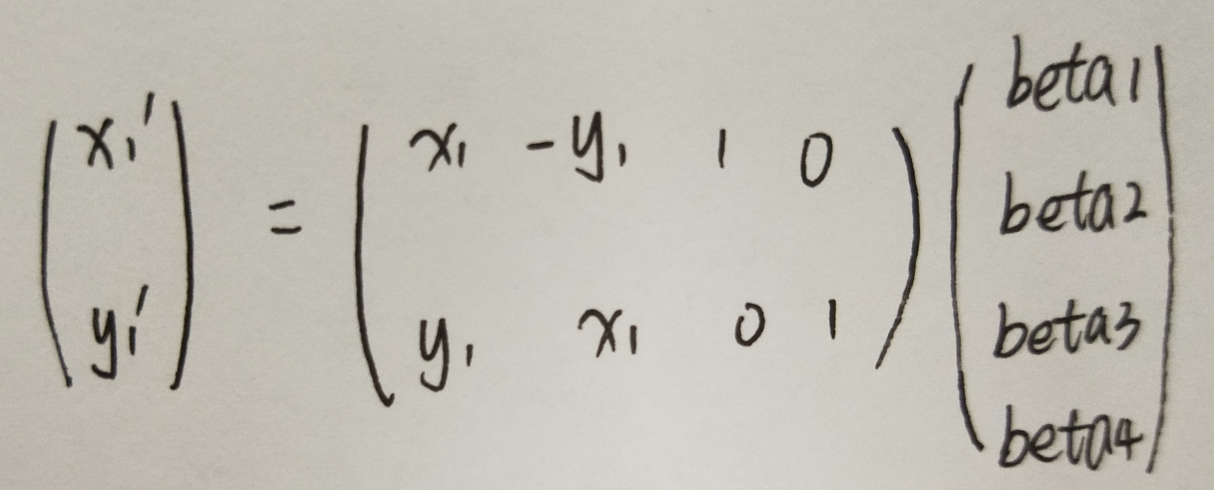
for idx = 1:size(x,2)
        A = [A; x(idx) -y(idx) 1 0;
                y(idx)  x(idx) 0 1];

        b = [b;x_(idx);
               y_(idx)];
    end
    beta = A\b;

    S_segment{i} = [beta(1) -beta(2) beta(3);
                    beta(2)  beta(1) beta(4);
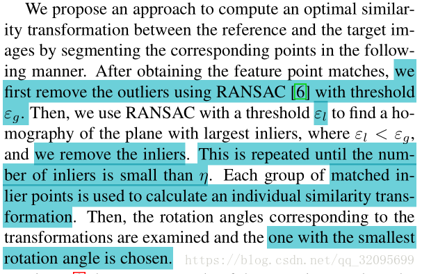
                         0        0       1];

ransac_global_similarity(data,data_orig,img1,img2)函数：
作用：查找旋转角度最小的相似矩阵

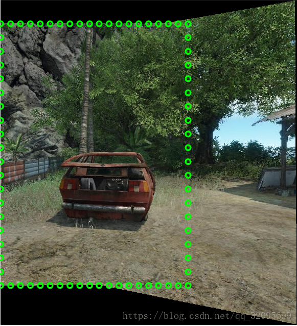
function S = ransac_global_similarity(data,data_orig,img1,img2)
thr_l = 0.001;
M = 500;

figure(1);
imshow([img1 img2]);
title('Ransac''s results');
hold on;
plot(data_orig(1,:),data_orig(2,:),'go','LineWidth',2);
plot(data_orig(4,:)+size(img1,2),data_orig(5,:),'go','LineWidth',2);
hold on;
pause(0.5)

%通过门限值thr_l获取内点inliers
for i = 1:20
    [ ~,res,~,~ ] = multigsSampling(100,data,M,10);
    con = sum(res<=thr_l);
    [ ~, maxinx ] = max(con);
    inliers = find(res(:,maxinx)<=thr_l);
    if size(inliers) < 50
        break;
    end
    data_inliers = data(:,inliers);

    x  = data_inliers(1,:); 
    y  = data_inliers(2,:); 
    x_ = data_inliers(4,:);     
    y_ = data_inliers(5,:);

    A = [];
    b = [];

    for idx = 1:size(x,2)
        A = [A; x(idx) -y(idx) 1 0;
                y(idx)  x(idx) 0 1];

        b = [b;x_(idx);
               y_(idx)];
    end
    beta = A\b;

    %通过inliers计算相似矩阵
    S_segment{i} = [beta(1) -beta(2) beta(3);
                    beta(2)  beta(1) beta(4);
                         0        0       1];
    %计算旋转角度                         
    theta(i)     = atan(beta(2)/beta(1));

    clr = [rand(),0,rand()];
    plot(data_orig(1,inliers),data_orig(2,inliers),...
         'o','color',clr,'LineWidth',2);
    plot(data_orig(4,inliers)+size(img1,2),data_orig(5,inliers),...
         'o','color',clr,'LineWidth',2);
    hold on;
    pause(0.5);

    %查找outliners,删除内点inliers
    outliers = find(res(:,maxinx)>thr_l);
    data = data(:,outliers);
    data_orig = data_orig(:,outliers);
end

index = find(abs(theta) == min(abs(theta)));
S = S_segment{index};
end

这一段代码对应论文：
这里写图片描述
for i = 1:20
……
end
循环：
i=1时：

相似矩阵S:
这里写图片描述
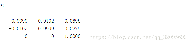
7、计算pano大小

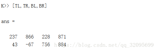
 %% Obtaining size of canvas (using global Homography).%img2映射到canvas的坐标-->H\x2
    TL = Hg\[1;1;1];
    TL = round([ TL(1)/TL(3) ; TL(2)/TL(3) ]);
    BL = Hg\[1;size(img2,1);1];
    BL = round([ BL(1)/BL(3) ; BL(2)/BL(3) ]);
    TR = Hg\[size(img2,2);1;1];
    TR = round([ TR(1)/TR(3) ; TR(2)/TR(3) ]);
    BR = Hg\[size(img2,2);size(img2,1);1];
    BR = round([ BR(1)/BR(3) ; BR(2)/BR(3) ]);

    % Canvas size.
    cw = max([1 size(img1,2) TL(1) BL(1) TR(1) BR(1)]) - min([1 size(img1,2) TL(1) BL(1) TR(1) BR(1)]) + 1;
    ch = max([1 size(img1,1) TL(2) BL(2) TR(2) BR(2)]) - min([1 size(img1,1) TL(2) BL(2) TR(2) BR(2)]) + 1;

    % Offset for left image.
    off = [ 1 - min([1 size(img1,2) TL(1) BL(1) TR(1) BR(1)]) + 1 ;
            1 - min([1 size(img1,1) TL(2) BL(2) TR(2) BR(2)]) + 1 ];

img2**映射前**的TL,BL,TR,BR如下图所示：
这里写图片描述
img2**映射后**的TL,BL,TR,BR：

8、把img1框起来

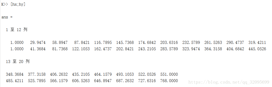
%% Generate anchor points in the boundary,20 in each size, 80 in total
anchor_points = [];
anchor_num = 20;
hx = linspace(1,size(img1,2),anchor_num);
hy = linspace(1,size(img1,1),anchor_num);

for i = 1:anchor_num
    anchor_points = [anchor_points;
                     1, round(hy(i))];    
    anchor_points = [anchor_points;
                     size(img1,2), round(hy(i))];   
    anchor_points = [anchor_points;
                     round(hx(i)), 1];    
    anchor_points = [anchor_points;
                     round(hx(i)), size(img1,1)];
end

将img1用为20*20的圆点框起来的网格
[hx;hy]:

这里写图片描述

9、计算权重

  %% Compute weight for Integration
       % (x,y): K_min -> K_1 -> K_2 -> K_max
    Or = [size(img1,2)/2;size(img1,1)/2];
    Ot = Hg\[size(img2,2)/2;size(img2,1)/2;1];
    Ot = [Ot(1)/Ot(3);Ot(2)/Ot(3)];

    % solve linear problem
    k = (Ot(2) - Or(2))/(Ot(1) - Or(1));%斜率
    b = Or(2) - k * Or(1);%截距

    K_min(1) = min([TL(1) BL(1) TR(1) BR(1)]);
    K_max(1) = max([TL(1) BL(1) TR(1) BR(1)]);
    K_1(1) = size(img1,2);
    K_2(1) = K_1(1) + (K_max(1) - K_1(1))/2;%img2投影后的中点横坐标

    K_min(2) = k * K_min(1) + b;
    K_max(2) = k * K_max(1) + b;
    K_1(2) = k * K_1(1) + b;
    K_2(2) = k * K_2(1) + b;

    % Image keypoints coordinates
    Kp = [data_orig(1,inliers)' data_orig(2,inliers)'];

    [ X,Y ] = meshgrid(linspace(1,cw,C1),linspace(1,ch,C2));

    % Mesh (cells) vertices' coordinates.
    Mv = [X(:)-off(1), Y(:)-off(2)];

    % Perform Moving DLT
    fprintf('  Moving DLT main loop...');tic;
    Ht = zeros(size(Mv,1),9);
    Hr = zeros(size(Mv,1),9);