TensorFlow实现CNN

TensorFlow是目前深度学习最流行的框架，很有学习的必要，下面我们就来实际动手，使用TensorFlow搭建一个简单的CNN，来对经典的mnist数据集进行数字识别。

step 0 导入TensorFlow

import tensorflow as tffrom tensorflow.examples.tutorials.mnist import input_data

step 1 加载数据集mnist

声明两个placeholder，用于存储神经网络的输入，输入包括image和label。这里加载的image是(784,)的shape。

mnist = input_data.read_data_sets('MNIST_data/', one_hot=True)
x = tf.placeholder(tf.float32,[None, 784])
y_ = tf.placeholder(tf.float32, [None, 10])

step 2 定义weights和bias

为了使代码整洁，这里把weight和bias的初始化封装成函数。

#----Weight Initialization---#
#One should generally initialize weights with a small amount of noise for symmetry breaking, and to prevent 0 gradients
def weight_variable(shape):
    initial = tf.truncated_normal(shape, stddev=0.1)
    return tf.Variable(initial)
def bias_variable(shape):
    initial = tf.constant(0.1, shape=shape)
    return tf.Variable(initial)

step 3 定义卷积层和maxpooling

同样，为了代码的整洁，将卷积层和maxpooling封装起来。padding=‘SAME’表示使用padding，不改变图片的大小。

#Convolution and Pooling
#Our convolutions uses a stride of one and are zero padded so that the output is the same size as the input.
#Our pooling is plain old max pooling over 2x2 blocks
def conv2d(x, W):
    return tf.nn.conv2d(x, W, strides=[1,1,1,1], padding='SAME')
def max_pool_2x2(x):
    return tf.nn.max_pool(x, ksize=[1,2,2,1], strides=[1,2,2,1], padding='SAME')

step 4 reshape image数据

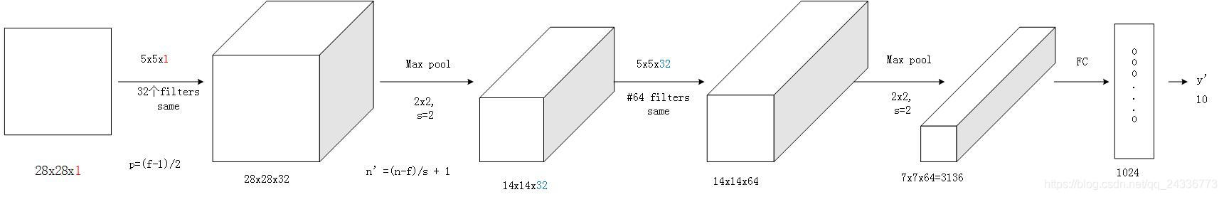
为了神经网络的layer可以使用image数据，我们要将其转化成4d的tensor: (Number, width, height, channels)

#To apply the layer, we first reshape x to a 4d tensor, with the second and third dimensions corresponding to image width and height,
#and the final dimension corresponding to the number of color channels.
x_image = tf.reshape(x, [-1,28,28,1])

step 5 搭建第一个卷积层

使用32个5x5的filter，然后通过maxpooling。

#----first convolution layer----#
#he convolution will compute 32 features for each 5x5 patch. Its weight tensor will have a shape of [5, 5, 1, 32].
#The first two dimensions are the patch size,
#the next is the number of input channels, and the last is the number of output channels.
W_conv1 = weight_variable([5,5,1,32])

#We will also have a bias vector with a component for each output channel.
b_conv1 = bias_variable([32])

#We then convolve x_image with the weight tensor, add the bias, apply the ReLU function, and finally max pool.
#The max_pool_2x2 method will reduce the image size to 14x14.
h_conv1 = tf.nn.relu(conv2d(x_image, W_conv1) + b_conv1)
h_pool1 = max_pool_2x2(h_conv1)

step 6 第二层卷积

使用64个5x5的filter。

#----second convolution layer----#
#The second layer will have 64 features for each 5x5 patch and input size 32.
W_conv2 = weight_variable([5,5,32,64])
b_conv2 = bias_variable([64])

h_conv2 = tf.nn.relu(conv2d(h_pool1, W_conv2) + b_conv2)
h_pool2 = max_pool_2x2(h_conv2)

step 7 构建全连接层

需要将上一层的输出，展开成1d的神经层。

#----fully connected layer----#
#Now that the image size has been reduced to 7x7, we add a fully-connected layer with 1024 neurons to allow processing on the entire image
W_fc1 = weight_variable([7*7*64, 1024])
b_fc1 = bias_variable([1024])

h_pool2_flat = tf.reshape(h_pool2, [-1, 7*7*64])
h_fc1 = tf.nn.relu(tf.matmul(h_pool2_flat,W_fc1) + b_fc1)

step 8 添加Dropout

加入Dropout层，可以防止过拟合问题。注意，这里使用了另外一个placeholder，可以控制在训练和预测时是否使用Dropout。

#-----dropout------#
#To reduce overfitting, we will apply dropout before the readout layer.
#We create a placeholder for the probability that a neuron's output is kept during dropout.
#This allows us to turn dropout on during training, and turn it off during testing.
keep_prob = tf.placeholder(tf.float32)
h_fc1_dropout = tf.nn.dropout(h_fc1, keep_prob)

step 9 输入层

没有什么特别的，就是输出一个线性结果。

#----read out layer----#
W_fc2 = weight_variable([1024,10])
b_fc2 = bias_variable([10])
y_conv = tf.matmul(h_fc1_dropout, W_fc2) + b_fc2

step 10 训练和评估

首先，需要指定一个cost function --cross_entropy，在输出层使用softmax。然后指定optimizer–adam。需要特别指出的是，一定要记得

tf.global_variables_initializer().run()初始化变量

#------train and evaluate----#
#计算成本
#tf.nn.softmax_cross_entropy_with_logits(labels=y_, logits=y_conv)：计算softmax的损失函数。这个函数既计算softmax的激活，也计算其损失；
#tf.reduce_mean：计算的是平均值，使用它来计算所有样本的损失来得到总成本。
cross_entropy = tf.reduce_mean(tf.nn.softmax_cross_entropy_with_logits(labels=y_, logits=y_conv))

##反向传播，由于框架已经实现了反向传播，我们只需要选择一个优化器就行了
train_step = tf.train.AdamOptimizer(1e-4).minimize(cross_entropy)

accuracy = tf.reduce_mean(tf.cast(tf.equal(tf.argmax(y_, 1), tf.argmax(y_conv, 1)), tf.float32))

with tf.Session() as sess:
    tf.global_variables_initializer().run()
    for i in range(3000):
        batch = mnist.train.next_batch(50)
        if i % 100 == 0:
            train_accuracy = accuracy.eval(feed_dict = {x: batch[0],
                                                       y_: batch[1],
                                                       keep_prob: 1.})
            print('setp {},the train accuracy: {}'.format(i, train_accuracy))
        train_step.run(feed_dict = {x: batch[0], y_: batch[1], keep_prob: 0.5})
    test_accuracy = accuracy.eval(feed_dict = {x: mnist.test.images, y_: mnist.test.labels, keep_prob: 1.})
    print('the test accuracy :{}'.format(test_accuracy))
    saver = tf.train.Saver()
    path = saver.save(sess, './my_net/mnist_deep.ckpt')
    print('save path: {}'.format(path))

运行一次挺慢的。
系统的整体架构与LeNet-5类似

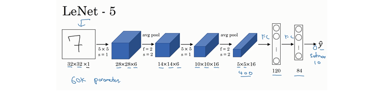
大致如下（个人理解，如有错误，还望各路大神指正）：

参考：https://www.cnblogs.com/yangmang/p/7528935.html#top
https://blog.youkuaiyun.com/cxmscb/article/details/71023576