智能股票分析与预测系统项目的开发

原创已于 2025-11-10 10:39:56 修改 · 867 阅读

16 ·

CC 4.0 BY-SA版权

文章标签：

#python #flask #scikit-learn #pandas #numpy #matplotlib #机器学习

于 2025-08-29 18:01:01 首次发布

智能股票分析预测系统是一个基于机器学习的股票分析与预测平台，集成了数据获取、特征工程、模型训练和可视化分析等功能。系统通过多种机器学习算法对股票历史数据进行分析，预测未来走势，并提供直观的可视化图表展示分析结果。

项目结构

📁 IntelligentStockAnalysisSystem/
- 📄 data_fetcher.py # 股票数据获取模块
- 📄 data_processor.py # 数据处理与特征工程
- 📄 feature_selector.py # 特征选择模块
- 📄 app.py # 程序入口
- 📄 model_trainer.py # 模型训练与评估
- 📄 visualizer.py # 可视化图表生成
- 📁 templates/ # HTML模板
  - 📄 dashboard.html # 主仪表盘页面
  - 📄 error.html # 错误页面
- 📁 static/ # 静态资源（CSS/JS/图片）
- 📄 README.md # 项目说明文档

功能特性

数据源支持：通过AKShare获取实时股票数据
高级特征工程：计算20+技术指标（MA、RSI、MACD、波动率等）
集成机器学习模型：随机森林、XGBoost、Lasso回归
时间序列验证：时间序列交叉验证
特征选择：基于相关性的特征筛选
可视化图表：生成8种专业分析图表
响应式Web界面：适配各种设备尺寸

快速开始

环境要求

Python 3.8+

安装步骤

安装依赖

pip install flask akshare pandas numpy scikit-learn xgboost matplotlib seaborn

运行项目

python app.py

在实现项目核心功能时，可以按照项目的运行流程来逐步实现对应的模块功能，其主要流程如图所示：

一、项目构建

开发项目前，需要完成项目初始化的设置，主要是项目运行所需的一些依赖库的安装。诸如，Flask、AkShare、Pandas、Scikit-learnFlask等。进行依赖的安装时，可以通过pip命令进行统一的安装。

# 统一安装项目运行所需的依赖

pip install flask akshare pandas numpy scikit-learn xgboost matplotlib seaborn

1.数据采集

股票数据采集函数完整的实现代码如下所示：

def get_stock_data(stock_code="600519", start_date="20000101", end_date=None):
    """
    获取股票历史数据
    """
    if end_date is None:
        # 默认结束日期为今天
        end_date = datetime.now().strftime("%Y%m%d")

    try:
        df = ak.stock_zh_a_hist(
            symbol=stock_code,
            period="daily",
            start_date=start_date,
            end_date=end_date,
            adjust="qfq"
        )

        # 如果数据为空，尝试其他数据源（并对备选数据源中的数据进行处理，使其列名与结构与主数据保持一致）
        if df.empty:
            df = ak.stock_zh_a_daily(symbol=stock_code, adjust="qfq")
            df = df.reset_index()
            df = df.rename(columns={'date': '日期', 'open': '开盘', 'close': '收盘',
                                    'high': '最高', 'low': '最低', 'volume': '成交量'})
            df = df[['日期', '开盘', '收盘', '最高', '最低', '成交量']]
        return df

    except Exception as e:
        print(f"获取数据失败: {e}")
        # 尝试备选数据源
        try:
            df = ak.stock_zh_a_daily(symbol=stock_code, adjust="qfq")
            df = df.reset_index()
            df = df.rename(columns={'date': '日期', 'open': '开盘', 'close': '收盘',
                                    'high': '最高', 'low': '最低', 'volume': '成交量'})
            df = df[['日期', '开盘', '收盘', '最高', '最低', '成交量']]
            return df
        except:
            # 返回空DataFrame
            return pd.DataFrame()

调用get_stock_data()函数，测试是否能正常获取股票数据，测试代码如下所示：

if __name__ == "__main__":

    code="600519"

    start_date="20000101"

    # 获取股票数据

    stock_data = get_stock_data(stock_code=code, start_date=start_date)

    print(stock_data)

运行效果如下所示：

              日期    股票代码       开盘       收盘  ...    振幅   涨跌幅    涨跌额   换手率

0     2020-01-02  600519   920.72   922.72  ...  2.98 -5.43 -53.00  1.18

1     2020-01-03  600519   909.72   871.28  ...  4.35 -5.57 -51.44  1.04

2     2020-01-06  600519   863.58   870.71  ...  2.94 -0.07  -0.57  0.50

3     2020-01-07  600519   870.22   887.25  ...  2.60  1.90  16.54  0.38

4     2020-01-08  600519   877.77   880.86  ...  1.46 -0.72  -6.39  0.20

...          ...     ...      ...      ...  ...   ...   ...    ...   ...

1329  2025-07-01  600519  1409.00  1405.10  ...  0.61 -0.31  -4.42  0.16

1330  2025-07-02  600519  1409.50  1409.60  ...  1.05  0.32   4.50  0.21

1331  2025-07-03  600519  1412.00  1415.60  ...  1.04  0.43   6.00  0.19

1332  2025-07-04  600519  1415.70  1422.22  ...  1.55  0.47   6.62  0.23

1333  2025-07-07  600519  1422.28  1410.70  ...  0.95 -0.81 -11.52  0.19



[1334 rows x 12 columns]

2.数据处理与特征工程

import pandas as pd
import numpy as np

def process_data(df, prediction_window=5):
    """数据清洗与特征工程"""
    # 重命名列
    df = df.rename(columns={
        '日期': 'date',
        '开盘': 'open',
        '收盘': 'close',
        '最高': 'high',
        '最低': 'low',
        '成交量': 'volume'
    })

    # 转换日期类型并设置索引
    df['date'] = pd.to_datetime(df['date'])
    df.set_index('date', inplace=True)

    # 添加基本技术指标
    df['ma5'] = df['close'].rolling(5, min_periods=1).mean()
    df['ma20'] = df['close'].rolling(20, min_periods=1).mean()
    df['ma60'] = df['close'].rolling(60, min_periods=1).mean()

    # 添加波动率指标
    df['daily_return'] = df['close'].pct_change()
    df['volatility_5d'] = df['daily_return'].rolling(5).std() * np.sqrt(252)
    df['volatility_20d'] = df['daily_return'].rolling(20).std() * np.sqrt(252)

    # 添加RSI和MACD
    df['rsi'] = compute_rsi(df['close'])
    df['macd'], df['signal'] = compute_macd(df['close'])

    # 添加成交量相关指标
    df['volume_ma5'] = df['volume'].rolling(5).mean()
    df['volume_ma20'] = df['volume'].rolling(20).mean()
    df['volume_ratio'] = df['volume'] / df['volume_ma20']

    # 添加时间特征
    df['year'] = df.index.year
    df['month'] = df.index.month
    df['day_of_week'] = df.index.dayofweek
    df['day_of_month'] = df.index.day

    # 添加滞后特征 计算当前时刻与过去 lag 天之间的收益率
    for lag in [1, 2, 3, 5, 10]:
        df[f'return_lag{lag}'] = df['close'].pct_change(lag)

    # 修改目标变量计算（未来几天的收益率） -计算当前时刻与未来 prediction_window 天之后的收盘价之间的收益率
    future_returns = df['close'].pct_change(prediction_window).shift(-prediction_window)

    # 使用滚动平均平滑目标变量
    smoothed_returns = future_returns.rolling(5, min_periods=1).mean()

    # 添加滞后特征作为目标变量
    df['future_return'] = smoothed_returns

    # 添加方向目标变量（用于分类）
    df['future_direction'] = np.where(df['future_return'] > 0, 1, 0)

    # 清理无效数据
    df.replace([np.inf, -np.inf], np.nan, inplace=True)
    df.dropna(inplace=True)

    # 验证数据
    validate_data(df)
    return df

def validate_data(df):
    """验证数据是否包含无效值"""
    # 首先检查空值
    if df.isnull().any().any():
        print(f"警告: 数据包含 {df.isnull().sum().sum()} 个空值")
        df.dropna(inplace=True)

    # 只检查数值列中的无穷值
    numeric_cols = df.select_dtypes(include=[np.number]).columns
    for col in numeric_cols:
        # 检查无穷值
        if np.isinf(df[col]).any():
            print(f"警告: 列 '{col}' 包含无穷值")
            # 替换无穷值为NaN
            df[col] = df[col].replace([np.inf, -np.inf], np.nan)

    # 再次检查空值（替换无穷值后可能产生新的空值）
    if df.isnull().any().any():
        print(f"警告: 数据替换后包含 {df.isnull().sum().sum()} 个空值")
        df.dropna(inplace=True)

    # 检查异常大值
    for col in numeric_cols:
        if (df[col].abs() > 1e10).any():
            print(f"警告: 列 '{col}' 包含异常大的数值")

    return df

3.MACD指标与RSI指标函数完整的实现代码如下所示：

def compute_rsi(series, period=14):

    """计算相对强弱指数RSI（添加边界条件处理）"""

    delta = series.diff()

    gain = delta.where(delta > 0, 0)

    loss = -delta.where(delta < 0, 0)



    # 避免除零错误

    avg_gain = gain.rolling(period, min_periods=1).mean()

    avg_loss = loss.rolling(period, min_periods=1).mean()



    # 添加额外保护：当avg_loss为0时直接返回100

    rs = avg_gain / avg_loss

    rs = np.where(avg_loss == 0, 100, rs)  # 当损失为0时，RS设为100



    rsi = 100 - (100 / (1 + rs))



    # 替换无效值

    rsi = pd.Series(rsi, index=series.index)

    rsi = rsi.fillna(50)  # 当数据不足时设为中性值50

    rsi.replace([np.inf, -np.inf], 50, inplace=True)



    return rsi



def compute_macd(series, fast=12, slow=26, signal=9):

    """计算MACD指标"""

    ema_fast = series.ewm(span=fast, min_periods=1).mean()

    ema_slow = series.ewm(span=slow, min_periods=1).mean()

    macd = ema_fast - ema_slow

    signal_line = macd.ewm(span=signal, min_periods=1).mean()

    return macd, signal_line

4.关键特征的筛选

在前面股票特征的构建过程中，设置了许多的特征，例如收盘价均线（ma5、ma20、ma60等）、成交量均线（volume_ma5、volume_ma20等）、MACD指标、RSI指标等。但是在模型的训练预测阶段，并不是所有的特征都能产生作用，可能有些特征对最终的预测结果影响较大，而一些特征对最终的预测结果影响较小。因此为了提高模型的性能，需要对特征进行筛选，尽量选取一些对最终预测结果影响较大的特征。

def select_features(df):
    """选择相关性高的特征"""
    # 计算特征与目标的相关性
    corr_matrix = df.corr()
    target_corr = corr_matrix['future_return'].abs().sort_values(ascending=False)

    # 选择相关性大于0.05的特征
    selected_features = target_corr[target_corr > 0.05].index.tolist()

    # 确保包含关键特征
    essential_features = [
        'close', 'volatility_20d', 'rsi', 'macd', 'volume_ratio',
        'year', 'ma5', 'ma20', 'daily_return', 'volume_ma5'
    ]
    for feat in essential_features:
        if feat not in selected_features and feat in df.columns:
            selected_features.append(feat)

    # 如果目标变量存在于筛选出的特征中移除目标变量
    if 'future_return' in selected_features:
        selected_features.remove('future_return')
    if 'future_direction' in selected_features:
        selected_features.remove('future_direction')

    return selected_features

5.模型的构建与训练

构建了随机森林、XGBoost和Lasso三种模型进行训练，并对它们的性能进行评估，从中确定性能最好的模型。

def train_and_evaluate_models(X, y):
    """训练多个模型并评估性能"""
    # 时间序列交叉验证
    tscv = TimeSeriesSplit(n_splits=5)
    # 构建模型字典
    models = {
        'RandomForest': RandomForestRegressor(
            n_estimators=200,
            max_depth=8,
            min_samples_leaf=15,
            max_features=0.7,
            random_state=42,
            n_jobs=-1
        ),
        'XGBoost': XGBRegressor(
            n_estimators=300,
            max_depth=5,
            learning_rate=0.03,
            subsample=0.7,
            colsample_bytree=0.8,
            random_state=42,
            n_jobs=-1
        ),
        'Lasso': LassoCV(cv=5, random_state=42, max_iter=10000)
    }

    #记录模型训练结果的字典
    results = {
        'model': [],
        'train_score': [],
        'test_score': [],
        'mae': []
    }
    # 记录最佳模型及其得分
    best_model = None
    best_score = -np.inf
    for model_name, model in models.items():
        fold_scores = []
        fold_mae = []
        for train_index, test_index in tscv.split(X):
            X_train, X_test = X.iloc[train_index], X.iloc[test_index]
            y_train, y_test = y.iloc[train_index], y.iloc[test_index]

            # 标准化 - 仅使用训练数据
            scaler = RobustScaler()
            X_train_scaled = scaler.fit_transform(X_train)
            X_test_scaled = scaler.transform(X_test)

            # 训练模型
            model.fit(X_train_scaled, y_train)

            # 评估模型
            train_score = model.score(X_train_scaled, y_train)
            test_score = model.score(X_test_scaled, y_test)
            y_pred = model.predict(X_test_scaled)
            mae = mean_absolute_error(y_test, y_pred)
            fold_scores.append(test_score)
            fold_mae.append(mae)

        # 计算平均性能
        avg_score = np.mean(fold_scores)
        avg_mae = np.mean(fold_mae)
        results['model'].append(model_name)
        results['train_score'].append(train_score)
        results['test_score'].append(avg_score)
        results['mae'].append(avg_mae)

        # 选择最佳模型
        if avg_score > best_score:
            best_score = avg_score
            best_model = model

    # 使用最近3年数据重新训练最佳模型
    recent_data = X[X.index.year >= datetime.now().year - 3]
    if not recent_data.empty:
        y_recent = y.loc[recent_data.index]
        scaler = RobustScaler()
        X_recent_scaled = scaler.fit_transform(recent_data)
        best_model.fit(X_recent_scaled, y_recent)
    return best_model, pd.DataFrame(results)

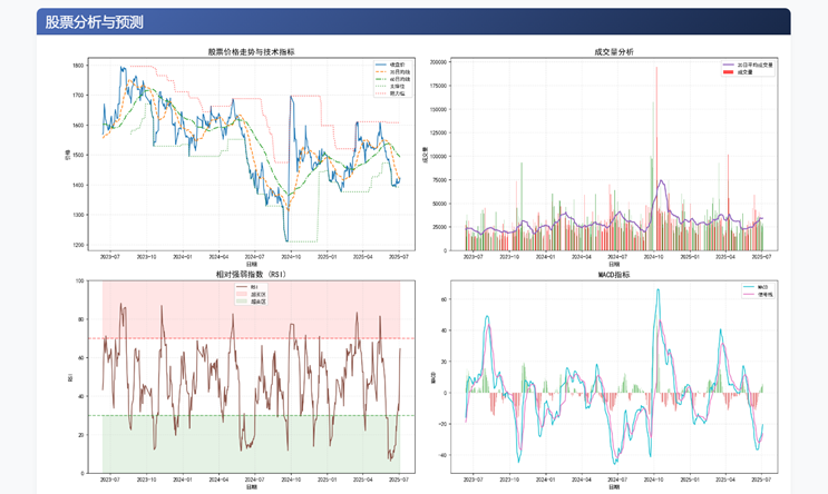
6.分析结果可视化

使用Matplotlib将模型的分析结果数据绘制为图表的形式方便用户进行数据分析。

def create_visualizations(df, model_performance, feature_importance):
    """生成股票分析可视化图表（优化版）"""
    # 第一部分：技术指标图表
    fig1 = plt.figure(figsize=(18, 22), constrained_layout=True)
    gs = fig1.add_gridspec(4, 2)

    # 1. 价格走势图（添加支撑/阻力线）
    ax1 = fig1.add_subplot(gs[0, 0])
    ax1.plot(df.index, df['close'], label='收盘价', linewidth=1.5, color='#1f77b4')
    ax1.plot(df.index, df['ma20'], label='20日均线', linestyle='--', color='#ff7f0e')
    ax1.plot(df.index, df['ma60'], label='60日均线', linestyle='-.', color='#2ca02c')

    # 添加支撑阻力线（示例逻辑，可根据实际需求调整）
    support = df['close'].rolling(50).min().dropna()
    resistance = df['close'].rolling(50).max().dropna()
    ax1.plot(support.index, support, 'g:', alpha=0.7, label='支撑位')
    ax1.plot(resistance.index, resistance, 'r:', alpha=0.7, label='阻力位')

    ax1.set_title('股票价格走势与技术指标', fontsize=14, fontweight='bold')
    ax1.set_xlabel('日期')
    ax1.set_ylabel('价格')
    ax1.legend(loc='best', fontsize=9)
    ax1.grid(True, linestyle='--', alpha=0.3)

    # 2. 成交量分析（添加颜色编码）
    ax2 = fig1.add_subplot(gs[0, 1])
    # 根据涨跌着色
    colors = np.where(df['close'].diff() >= 0, 'g', 'r')
    ax2.bar(df.index, df['volume'], color=colors, alpha=0.7, label='成交量')
    ax2.plot(df.index, df['volume_ma20'], color='#9467bd', linewidth=2, label='20日平均成交量')
    ax2.set_title('成交量分析', fontsize=14, fontweight='bold')
    ax2.set_xlabel('日期')
    ax2.set_ylabel('成交量')
    ax2.legend(loc='best', fontsize=9)
    ax2.grid(True, linestyle='--', alpha=0.3)

    # 3. RSI指标（添加超买超卖区域）
    ax3 = fig1.add_subplot(gs[1, 0])
    ax3.plot(df.index, df['rsi'], label='RSI', color='#8c564b', linewidth=1.5)
    ax3.axhline(70, color='red', linestyle='--', alpha=0.5)
    ax3.axhline(30, color='green', linestyle='--', alpha=0.5)
    ax3.fill_between(df.index, 70, 100, color='red', alpha=0.1, label='超买区')
    ax3.fill_between(df.index, 0, 30, color='green', alpha=0.1, label='超卖区')
    ax3.set_title('相对强弱指数 (RSI)', fontsize=14, fontweight='bold')
    ax3.set_xlabel('日期')
    ax3.set_ylabel('RSI')
    ax3.set_ylim(0, 100)
    ax3.legend(loc='best', fontsize=9)
    ax3.grid(True, linestyle='--', alpha=0.3)

    # 4. MACD指标（优化柱状图显示）
    ax4 = fig1.add_subplot(gs[1, 1])
    ax4.plot(df.index, df['macd'], label='MACD', color='#17becf', linewidth=1.5)
    ax4.plot(df.index, df['signal'], label='信号线', color='#e377c2', linewidth=1.5)
    # 使用更高效的bar绘制方法
    diff = df['macd'] - df['signal']
    ax4.bar(df.index, diff, color=np.where(diff > 0, '#2ca02c', '#d62728'), alpha=0.5, width=1)
    ax4.set_title('MACD指标', fontsize=14, fontweight='bold')
    ax4.set_xlabel('日期')
    ax4.set_ylabel('MACD')
    ax4.legend(loc='best', fontsize=9)
    ax4.grid(True, linestyle='--', alpha=0.3)

    # 5. 波动率分析（添加布林带）
    ax5 = fig1.add_subplot(gs[2, 0])
    ax5.plot(df.index, df['volatility_20d'] * 100, label='20日波动率', color='#bcbd22', linewidth=1.5)
    ax5.set_title('波动率分析', fontsize=14, fontweight='bold')
    ax5.set_xlabel('日期')
    ax5.set_ylabel('波动率 (%)')
    ax5.legend(loc='best', fontsize=9)
    ax5.grid(True, linestyle='--', alpha=0.3)

    # 6. 模型性能比较（添加具体数值标签）
    ax6 = fig1.add_subplot(gs[2, 1])
    bars = ax6.bar(model_performance['model'], model_performance['test_score'],
                   color=['#1f77b4', '#ff7f0e', '#2ca02c'])
    ax6.set_title('模型性能比较 (测试集$R^2$得分)', fontsize=14, fontweight='bold')
    ax6.set_ylabel('$R^2$得分')
    ax6.grid(True, linestyle='--', alpha=0.3)

    # 在柱状图上添加数值标签
    for bar in bars:
        height = bar.get_height()
        ax6.annotate(f'{height:.3f}',
                     xy=(bar.get_x() + bar.get_width() / 2, height),
                     xytext=(0, 3),  # 3 points vertical offset
                     textcoords="offset points",
                     ha='center', va='bottom', fontsize=9)

    # 7. 特征重要性（优化显示）
    ax7 = fig1.add_subplot(gs[3, 0])
    top_features = feature_importance.head(10).sort_values(by='importance', ascending=True)
    colors = plt.cm.viridis(np.linspace(0, 1, len(top_features)))
    ax7.barh(top_features['feature'], top_features['importance'], color=colors)
    ax7.set_title('Top 10特征重要性', fontsize=14, fontweight='bold')
    ax7.set_xlabel('重要性')
    ax7.grid(True, linestyle='--', alpha=0.3)

    # 8. 预测与实际对比（添加回归线和R²）
    ax8 = fig1.add_subplot(gs[3, 1])
    ax8.scatter(df['future_return'], df['prediction'], alpha=0.5, color='#d62728', s=20)

    # 添加回归线
    slope, intercept = np.polyfit(df['future_return'], df['prediction'], 1)
    regression_line = slope * df['future_return'] + intercept
    ax8.plot(df['future_return'], regression_line, 'b-', linewidth=2, label=f'回归线 (斜率={slope:.2f})')

    # 添加45度参考线
    ax8.plot([df['future_return'].min(), df['future_return'].max()],
             [df['future_return'].min(), df['future_return'].max()],
             'r--', linewidth=1.5, label='理想线')

    # 计算R²
    r2 = r2_score(df['future_return'], df['prediction'])
    ax8.annotate(f'$R^2$ = {r2:.3f}', xy=(0.05, 0.9), xycoords='axes fraction', fontsize=12)
    ax8.set_xlabel('实际收益率')
    ax8.set_ylabel('预测收益率')
    ax8.set_title('预测 vs 实际', fontsize=14, fontweight='bold')
    ax8.legend(loc='best', fontsize=9)
    ax8.grid(True, linestyle='--', alpha=0.3)

    # 保存为Base64编码
    buffer1 = BytesIO()
    fig1.savefig(buffer1, format='png', dpi=120, bbox_inches='tight')
    buffer1.seek(0)
    img_base64 = base64.b64encode(buffer1.read()).decode()
    plt.close(fig1)  # 明确关闭图形释放内存

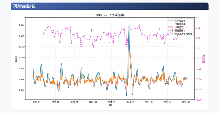
    # 第二部分：诊断图 - 实际vs预测的时间序列对比
    fig2, ax = plt.subplots(figsize=(12, 6), tight_layout=True)

    # 绘制实际和预测值
    ax.plot(df.index, df['future_return'], label='实际收益率', color='#1f77b4', linewidth=1.5)
    ax.plot(df.index, df['prediction'], label='预测收益率', color='#ff7f0e', linewidth=1.5)

    # 添加残差区域
    ax.fill_between(df.index, df['future_return'], df['prediction'],
                    where=(df['prediction'] > df['future_return']),
                    color='red', alpha=0.2, label='预测高估')
    ax.fill_between(df.index, df['future_return'], df['prediction'],
                    where=(df['prediction'] <= df['future_return']),
                    color='green', alpha=0.2, label='预测低估')

    # 添加滚动相关系数
    rolling_corr = df['future_return'].rolling(30).corr(df['prediction'])
    ax2 = ax.twinx()
    ax2.plot(df.index, rolling_corr, 'm--', alpha=0.7, label='30日滚动相关系数')
    ax2.set_ylabel('相关系数', color='m')
    ax2.tick_params(axis='y', labelcolor='m')
    ax2.set_ylim(-1, 1)
    ax.set_title('实际 vs 预测收益率', fontsize=14, fontweight='bold')
    ax.set_xlabel('日期')
    ax.set_ylabel('收益率')

    # 合并图例
    lines, labels = ax.get_legend_handles_labels()
    lines2, labels2 = ax2.get_legend_handles_labels()
    ax.legend(lines + lines2, labels + labels2, loc='best')
    ax.grid(True, linestyle='--', alpha=0.3)

    # 保存为Base64编码
    buffer2 = BytesIO()
    fig2.savefig(buffer2, format='png', dpi=120, bbox_inches='tight')
    buffer2.seek(0)
    diag_img = base64.b64encode(buffer2.read()).decode()
    plt.close(fig2)  # 明确关闭图形释放内存

    return img_base64, diag_img

7.web交互

为了给用户提供一个良好的交互体验，我们可以借助Flask框架快速构建一个后端服务器，用来监听用户请求，并调用业务代码完成股票数据的查询、处理、模型性训练以及数据分析的完整流程，最终将分析结果返回到前端HTML页面中，实现前后端数据的交互。

from flask import Flask, render_template, request
import traceback
from datetime import datetime
from data_fetcher import get_stock_data
from data_processor import process_data
from feature_selector import select_features
from model_trainer import train_and_evaluate_models, get_feature_importance
from visualizer import create_visualizations
from sklearn.preprocessing import RobustScaler

# 实例化一个Flask框架应用
app = Flask(__name__)

@app.route('/', methods=['GET', 'POST'])
def stock_analysis():
    print("表单提交内容:", request.form)
    if request.method == 'POST':
        stock_code = request.form.get('stock_code', '600519')
        start_date = request.form.get('start_date', '20200101')
        prediction_window = int(request.form.get('prediction_window', '5'))
    else:
        stock_code = "600519"
        start_date = "20200101"
        prediction_window = 5
    print(start_date,'开始时间')
    # 默认结束日期为今天
    end_date = datetime.now().strftime("%Y%m%d")
    if start_date >= end_date:
        return render_template("error.html", message="起始日期不能大于等于结束日期")
    try:
        # 获取并处理数据
        df = get_stock_data(stock_code, start_date=start_date,end_date=end_date)
        if df.empty:
            return render_template('error.html', message="无法获取股票数据，请检查股票代码是否正确")
        # 构建特征
        processed_df = process_data(df, prediction_window)

        # 特征选择
        features = select_features(processed_df)
        X = processed_df[features]
        y = processed_df['future_return']

        # 训练模型并评估
        model, model_performance = train_and_evaluate_models(X, y)

        # 在完整数据集上生成预测
        scaler = RobustScaler()
        X_scaled = scaler.fit_transform(X)
        processed_df['prediction'] = model.predict(X_scaled)

        # 获取特征重要性
        feature_imp = get_feature_importance(model, features)

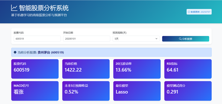
        # 关键指标计算
        latest = processed_df.iloc[-1]
        metrics = {
            "股票代码": stock_code,
            "当前价格": f"{latest['close']:.2f}",
            "20日波动率": f"{latest['volatility_20d'] * 100:.2f}%",
            "RSI指标": f"{latest['rsi']:.2f}",
            "MACD信号": "看涨" if latest['macd'] > latest['signal'] else "看跌",
            f"未来{prediction_window}日预期收益": f"{latest['prediction'] * 100:.2f}%",
            "最佳模型": model_performance.loc[model_performance['test_score'].idxmax(), 'model'],
            "模型测试得分": f"{model_performance['test_score'].max():.3f}"
        }

        # 模型性能表格
        model_table = model_performance.to_dict('records')
        # 特征重要性表格
        feature_table = feature_imp.head(10).to_dict('records')
        # 生成可视化图表
        plot_img, diag_img = create_visualizations(processed_df.tail(500), model_performance, feature_imp)

        # 获取股票名称
        try:
            import akshare as ak
            stock_info = ak.stock_individual_info_em(symbol=stock_code)
            stock_name = stock_info.loc[stock_info['item'] == '股票简称', 'value'].values[0]
            print(stock_name)
        except:
            stock_name = "未知股票"
        # 返回股票分析HTML页面，并将数据嵌入页面中
        return render_template('dashboard.html',
                               plot=plot_img,# 股票分析与预测股票图片
                               diag_plot=diag_img,# 股票预测性能诊断图片
                               metrics=metrics,# 股票分析指标
                               model_table=model_table,# 模型性能表格
                               feature_table=feature_table,# 特征重要性表格
                               stock_name=stock_name,# 股票名称
                               prediction_window=prediction_window,# 预测窗口
                               start_date=start_date,# 开始日期
                               current_date=end_date,# 当前日期
                               stock_code=stock_code)# 股票代码

    except Exception as e:
        error_trace = traceback.format_exc()
        return render_template('error.html', message=str(e), trace=error_trace)


# 错误处理页面
@app.errorhandler(404)
def page_not_found(e):
    return render_template('error.html', message="页面未找到"), 404


@app.errorhandler(500)
def internal_server_error(e):
    error_trace = traceback.format_exc()
    return render_template('error.html', message="服务器内部错误", trace=error_trace), 500

# 程序主入口，运行Flask框架
if __name__ == "__main__":
    app.run(debug=True)

项目运行效果图：