


目录
八、批量标准化
批量标准化(Batch Normalization, BN)是一种广泛使用的神经网络正则化技术,核心思想是对每一层的输入进行标准化,然后进行缩放和平移,旨在加速训练、提高模型的稳定性和泛化能力。批量标准化通常在全连接层或卷积层之后、激活函数之前应用。
核心思想
Batch Normalization(BN)通过对每一批(batch)数据的每个特征通道进行标准化,解决内部协变量偏移(Internal Covariate Shift)问题,从而:
-
加速网络训练
-
允许使用更大的学习率
-
减少对初始化的依赖
-
提供轻微的正则化效果
批量标准化的基本思路是在每一层的输入上执行标准化操作,并学习两个可训练的参数:缩放因子 和偏移量
。
在深度学习中,批量标准化(Batch Normalization)在训练阶段和测试阶段的行为是不同的。在测试阶段,由于没有 mini-batch 数据,无法直接计算当前 batch 的均值和方差,因此需要使用训练阶段计算的全局统计量(均值和方差)来进行标准化。
官网地址:torch.nn — PyTorch 2.8 documentation
1. 训练阶段的批量标准化
1.1 计算均值和方差
对于给定的神经网络层,假设输入数据为 ,其中 m是批次大小。我们首先计算该批次数据的均值和方差。
-
均值(Mean)
$$
\mu_B = \frac{1}{m} \sum_{i=1}^m x_i
$$ -
方差
$$
\sigma_B^2 = \frac{1}{m} \sum_{i=1}^m (x_i - \mu_B)^2
$$
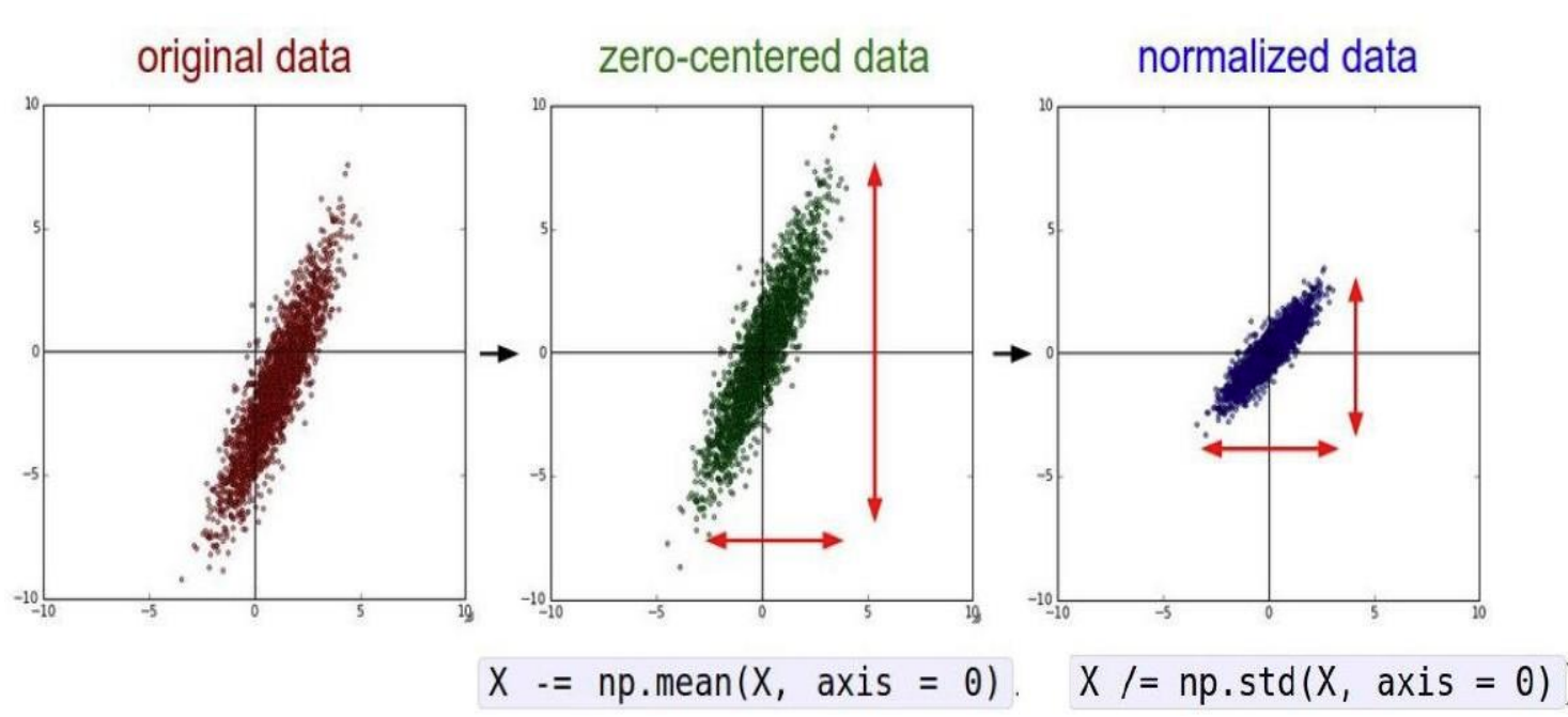
1.2 标准化
使用计算得到的均值和方差对数据进行标准化,使得每个特征的均值为0,方差为1。
-
标准化后的值
$$
\hat{x}_i = \frac{x_i - \mu_B}{\sqrt{\sigma_B^2 + \epsilon}}
$$其中,
是一个很小的常数,防止除以零的情况。
1.3 缩放和平移
标准化后的数据通常会通过可训练的参数进行缩放和平移,以恢复模型的表达能力。
-
缩放(Gamma):
$$
y_i = \gamma \hat{x}_i
$$ -
平移(Beta):
$$
y_i = \gamma \hat{x}_i + \beta
$$其中,
和
是在训练过程中学习到的参数。它们会随着网络的训练过程通过反向传播进行更新。
1.4 更新全局统计量
通过指数移动平均(Exponential Moving Average, EMA)更新全局均值和方差:
$$
μ_{global}=(1−momentum)⋅μ_{global}+momentum⋅μ_B\\ σ_{global}^2=(1−momentum)⋅σ_{global}^2+momentum⋅σ_B^2
$$
其中,momentum 是一个超参数,控制当前 mini-batch 统计量对全局统计量的贡献。
momentum 是一个介于 0 和 1 之间的值,控制当前 mini-batch 统计量的权重。PyTorch 中 momentum 的默认值是 0.1。
与优化器中的 momentum 的区别
-
批量标准化中的 momentum:
-
用于更新全局统计量(均值和方差)。
-
控制当前 mini-batch 统计量对全局统计量的贡献。
-
-
优化器中的 momentum:
-
用于加速梯度下降过程,帮助跳出局部最优。
-
例如,SGD 优化器中的 momentum 参数。
-
两者虽然名字相同,但作用完全不同,不要混淆。
2. 测试阶段的批量标准化
在测试阶段,由于没有 mini-batch 数据,无法直接计算当前 batch 的均值和方差。因此,使用训练阶段通过 EMA 计算的全局统计量(均值和方差)来进行标准化。
在测试阶段,使用全局统计量对输入数据进行标准化:
$$
\hat x_i=\frac{x_i−μ_{global}}{\sqrt{σ_{global}^2+ϵ}}
$$
然后对标准化后的数据进行缩放和平移:
$$
yi=γ⋅\hat{x}_i+β
$$
为什么使用全局统计量?
一致性:
-
在测试阶段,输入数据通常是单个样本或少量样本,无法准确计算均值和方差。
-
使用全局统计量可以确保测试阶段的行为与训练阶段一致。
稳定性:
-
全局统计量是通过训练阶段的大量 mini-batch 数据计算得到的,能够更好地反映数据的整体分布。
-
使用全局统计量可以减少测试阶段的随机性,使模型的输出更加稳定。
效率:
-
在测试阶段,使用预先计算的全局统计量可以避免重复计算,提高效率。
3. 作用
批量标准化(Batch Normalization, BN)通过以下几个方面来提高神经网络的训练稳定性、加速训练过程并减少过拟合:
3.1 缓解梯度问题
标准化处理可以防止激活值过大或过小,避免了激活函数(如 Sigmoid 或 Tanh)饱和的问题,从而缓解梯度消失或爆炸的问题。
3.2 加速训练
由于 BN 使得每层的输入数据分布更为稳定,因此模型可以使用更高的学习率进行训练。这可以加快收敛速度,并减少训练所需的时间。
3.3 减少过拟合
-
类似于正则化:虽然 BN 不是一种传统的正则化方法,但它通过对每个批次的数据进行标准化,可以起到一定的正则化作用。它通过在训练过程中引入了噪声(由于批量均值和方差的估计不完全准确),这有助于提高模型的泛化能力。
-
避免对单一数据点的过度拟合:BN 强制模型在每个批次上进行标准化处理,减少了模型对单个训练样本的依赖。这有助于模型更好地学习到数据的整体特征,而不是对特定样本的噪声进行过度拟合。
4.函数说明
torch.nn.BatchNorm1d 是 PyTorch 中用于一维数据的批量标准化(Batch Normalization)模块。
 torch.nn.BatchNorm1d(
     num_features,         # 输入数据的特征维度
     eps=1e-05,           # 用于数值稳定性的小常数
     momentum=0.1,        # 用于计算全局统计量的动量
     affine=True,         # 是否启用可学习的缩放和平移参数
     track_running_stats=True,  # 是否跟踪全局统计量
     device=None,         # 设备类型(如 CPU 或 GPU)
     dtype=None           # 数据类型
 )
参数说明:
eps:用于数值稳定性的小常数,添加到方差的分母中,防止除零错误。默认值:1e-05
momentum:用于计算全局统计量(均值和方差)的动量。默认值:0.1,参考本节1.4
affine:是否启用可学习的缩放和平移参数(γ和 β)。如果 affine=True,则模块会学习两个参数;如果 affine=False,则不学习参数,直接输出标准化后的值 。默认值:True
track_running_stats:是否跟踪全局统计量(均值和方差)。如果 track_running_stats=True,则在训练过程中计算并更新全局统计量,并在测试阶段使用这些统计量。如果 track_running_stats=False,则不跟踪全局统计量,每次标准化都使用当前 mini-batch 的统计量。默认值:True
4. 代码实现
import torch
from torch import nn
from matplotlib import pyplot as plt
from sklearn.datasets import make_circles
from sklearn.model_selection import train_test_split
from torch.nn import functional as F
from torch import optim
# 数据准备
# 生成非线性可分数据(同心圆)
# n_samples int 总样本数(默认100),内外圆各占一半
# noise float 添加到数据中的高斯噪声标准差(默认0.0)
# factor float 内圆与外圆的半径比(默认0.8)
# random_state int 随机数种子,保证可重复性
# 输出数据
# X: 二维坐标数组,形状 (n_samples, 2)
# 每行是一个数据点的 [x, y] 坐标
# y: 类别标签 0(外圆)或 1(内圆),形状 (n_samples,)
x, y = make_circles(n_samples=2000, noise=0.1, factor=0.4, random_state=42)
x = torch.tensor(x, dtype=torch.float)
y = torch.tensor(y, dtype=torch.long)
x_train, x_test, y_train, y_test = train_test_split(x, y, test_size=0.3, random_state=42)
# 可视化原始训练数据和测试数据
plt.scatter(x[:, 0], x[:, 1], c=y, cmap='coolwarm', edgecolors='k')
plt.show()
# 定义BN模型
class NetWithBN(nn.Module):
def __init__(self):
super().__init__()
self.fc1 = nn.Linear(2, 64)
self.bn1 = nn.BatchNorm1d(64)
self.fc2 = nn.Linear(64, 32)
self.bn2 = nn.BatchNorm1d(32)
self.fc3 = nn.Linear(32, 2)
def forward(self, x):
x = F.relu(self.bn1(self.fc1(x)))
x = F.relu(self.bn2(self.fc2(x)))
x = self.fc3(x)
return x
# 定义无BN模型
class NetWithoutBN(nn.Module):
def __init__(self):
super().__init__()
self.fc1 = nn.Linear(2, 64)
self.fc2 = nn.Linear(64, 32)
self.fc3 = nn.Linear(32, 2)
def forward(self, x):
x = F.relu(self.fc1(x))
x = F.relu(self.fc2(x))
x = self.fc3(x)
return x
# 定义训练函数
def train(model, x_train, y_train, x_test, y_test, name, lr=0.1, epochs=500):
criterion = nn.CrossEntropyLoss()
optimizer = optim.SGD(model.parameters(), lr=lr)
train_loss = []
test_acc = []
for epoch in range(epochs):
model.train()
y_pred = model(x_train)
loss = criterion(y_pred, y_train)
optimizer.zero_grad()
loss.backward()
optimizer.step()
train_loss.append(loss.item())
model.eval()
with torch.no_grad():
y_test_pred = model(x_test)
_, pred = torch.max(y_test_pred, dim=1)
correct = (pred == y_test).sum().item()
test_acc.append(correct / len(y_test))
if epoch % 100 == 0:
print(f'{name}|Epoch:{epoch},loss:{loss.item():.4f},acc:{test_acc[-1]:.4f}')
return train_loss, test_acc
model_bn = NetWithBN()
model_nobn = NetWithoutBN()
bn_train_loss, bn_test_acc = train(model_bn, x_train, y_train, x_test, y_test, name='BN')
nobn_train_loss, nobn_test_acc = train(model_nobn, x_train, y_train, x_test, y_test, name='NoBN')
def plot(bn_train_loss, nobn_train_loss, bn_test_acc, nobn_test_acc):
fig = plt.figure(figsize=(12, 5))
ax1 = fig.add_subplot(1, 2, 1)
ax1.plot(bn_train_loss, 'b', label='BN')
ax1.plot(nobn_train_loss, 'r', label='NoBN')
ax1.legend()
ax2 = fig.add_subplot(1, 2, 2)
ax2.plot(bn_test_acc, 'b', label='BN')
ax2.plot(nobn_test_acc, 'r', label='NoBN')
ax2.legend()
plt.show()
plot(bn_train_loss, nobn_train_loss, bn_test_acc, nobn_test_acc)
九、模型的保存和加载
训练一个模型通常需要大量的数据、时间和计算资源。通过保存训练好的模型,可以满足后续的模型部署、模型更新、迁移学习、训练恢复等各种业务需要求。
1. 标准网络模型构建
class MyModle(nn.Module): def __init__(self, input_size, output_size): super(MyModle, self).__init__() # 创建一个全连接网络(full connected layer) self.fc1 = nn.Linear(input_size, 128) self.fc2 = nn.Linear(128, 64) self.fc3 = nn.Linear(64, output_size) def forward(self, x): x = self.fc1(x) x = self.fc2(x) output = self.fc3(x) return output # 创建模型实例 model = MyModel(input_size=10, output_size=2) # 输入数据 x = torch.randn(5, 10) # 调用模型 output = model(x)
forward 方法是 PyTorch 中 nn.Module 类的必须实现的方法。它是定义神经网络前向传播逻辑的地方,决定了数据如何通过网络层传递并生成输出。同时forward 方法定义了计算图,PyTorch 会根据这个计算图自动计算梯度并更新参数。
2. 序列化模型对象
模型序列化对象的保存和加载:
模型保存:
torch.save(obj, f, pickle_module=pickle, pickle_protocol=DEFAULT_PROTOCOL, _use_new_zipfile_serialization=True)
参数说明:
-
obj:要保存的对象,可以是模型、张量、字典等。
-
f:保存文件的路径或文件对象。可以是字符串(文件路径)或文件描述符。
-
pickle_module:用于序列化的模块,默认是 Python 的 pickle 模块。
-
pickle_protocol:pickle 模块的协议版本,默认是 DEFAULT_PROTOCOL(通常是最高版本)。
模型加载:
torch.load(f, map_location=None, pickle_module=pickle, **pickle_load_args)
参数说明:
-
f:文件路径或文件对象。可以是字符串(文件路径)或文件描述符。
-
map_location:指定加载对象的设备位置(如 CPU 或 GPU)。默认是 None,表示保持原始设备位置。例如:map_location=torch.device('cpu') 将对象加载到 CPU。
-
pickle_module:用于反序列化的模块,默认是 Python 的 pickle 模块。
-
pickle_load_args:传递给 pickle_module.load() 的额外参数。
import torch
import torch.nn as nn
import pickle
class MyModle(nn.Module):
def __init__(self, input_size, output_size):
super(MyModle, self).__init__()
self.fc1 = nn.Linear(input_size, 128)
self.fc2 = nn.Linear(128, 64)
self.fc3 = nn.Linear(64, output_size)
def forward(self, x):
x = self.fc1(x)
x = self.fc2(x)
output = self.fc3(x)
return output
def test001():
model = MyModle(input_size=128, output_size=32)
# 序列化方式保存模型对象
torch.save(model, "model.pkl", pickle_module=pickle, pickle_protocol=2)
def test002():
# 注意设备问题
model = torch.load("model.pkl", map_location="cpu", pickle_module=pickle)
print(model)
if __name__ == "__main__":
test001()
test002()
打印结果:
 MyModle(
   (fc1): Linear(in_features=128, out_features=128, bias=True)
   (fc2): Linear(in_features=128, out_features=64, bias=True)
   (fc3): Linear(in_features=64, out_features=32, bias=True)
 )
.pkl 文件是二进制文件,内容是通过 pickle 模块序列化的 Python 对象。它可以保存几乎任何 Python 对象,但可能存在兼容性问题(如 Python 2 和 Python 3 之间的差异)。
.pth 文件是二进制文件,内容通常是序列化的 PyTorch 模型或张量。使用 .pth 作为扩展名是为了明确表示这是一个 PyTorch 模型文件。
3. 保存模型参数
这种形式更常用,只需要保存权重、偏置、准确率等相关参数,都可以在加载后打印观察!
import torch
import torch.nn as nn
import torch.optim as optim
import pickle
class MyModle(nn.Module):
def __init__(self, input_size, output_size):
super(MyModle, self).__init__()
self.fc1 = nn.Linear(input_size, 128)
self.fc2 = nn.Linear(128, 64)
self.fc3 = nn.Linear(64, output_size)
def forward(self, x):
x = self.fc1(x)
x = self.fc2(x)
output = self.fc3(x)
return output
def test003():
model = MyModle(input_size=128, output_size=32)
optimizer = optim.SGD(model.parameters(), lr=0.01)
# 构建要存储的模型参数
save_dict = {
"init_params": {
"input_size": 128, # 输入特征数
"output_size": 32, # 输出特征数
},
"accuracy": 0.99, # 模型准确率
"model_state_dict": model.state_dict(),
"optimizer_state_dict": optimizer.state_dict(),
}
torch.save(save_dict, "model_dict.pth")
def test004():
save_dict = torch.load("model_dict.pth")
model = MyModle(
input_size=save_dict["init_params"]["input_size"],
output_size=save_dict["init_params"]["output_size"],
)
# 初始化模型参数
model.load_state_dict(save_dict["model_state_dict"])
optimizer = optim.SGD(model.parameters(), lr=0.01)
# 初始化优化器参数
optimizer.load_state_dict(save_dict["optimizer_state_dict"])
# 打印模型信息
print(save_dict["accuracy"])
print(model)
if __name__ == "__main__":
test003()
test004()
推理时加载模型参数简单如下:
# 保存模型状态字典
torch.save(model.state_dict(), 'model.pth')
# 加载模型状态字典
model = MyModel(128, 32)
model.load_state_dict(torch.load('model.pth'))
技术分享是一个相互学习的过程。关于本文的主题,如果你有不同的见解、发现了文中的错误,或者有任何不清楚的地方,都请毫不犹豫地在评论区留言。我很期待能和大家一起讨论,共同补充更多细节。


 8万+
8万+

 被折叠的 条评论
为什么被折叠?
被折叠的 条评论
为什么被折叠?
 到【灌水乐园】发言


