PyTorch：tensor-数学API

乘法API

一维tensor相乘：torch.dot

这个只支持一维相同维度的向量相乘，不支持2维以上。

torch.dot(torch.tensor([2, 3]), torch.tensor([2, 1]))

Note: np.dot就有点类似下面的matmul，和torch.dot完全不一样。

[TORCH.DOT]

二维tensor相乘：torch.mm

a是 [m, k]，b是[k, n]，结果是 [m, n]
c = torch.mm(a, b)

三维tensor相乘torch.bmm

c = torch.bmm(a, b)

只能用于三维tensor相乘，这个函数不支持广播，也就是第一维必须相同，另外两维符合矩阵相乘法则。

示例：实现A=ab,B=abc到ac，即a1b*abc=a1c

torch.bmm(A.unsqueeze(1),B).squeeze(1)

等价于torch.einsum("ab,abc->ac", A, B)

任意多维tensor相乘：torch.matmul

等价于@运算符。

支持广播；当两个都是一维时，表示点积
c = torch.matmul(a, b)

广播的意思同numpy，如ab维度为[1,2,1152,1,8][10,1,1152,8,16]，则matmul结果c的维度为[10,2,1152,1,16]，即只有最后两维会执行一一的矩阵运算，其它都是取有维度的那个（注意必须是两个维度一样大，或者其中一个是1，否则没法一一矩阵运算了，实际就是把1维变成了另一个维度大小且元素和1维一样）。

另外，如下例，[2,3,1]和[2,1,3]的结果维度是[2,3,3]。

利用这个可以实现规避batch维度功能，如想实现[揭秘 Deep & Cross : 如何自动构造高阶交叉特征 - 知乎]中x0*x0^t*w0，假如inputs = batch*feature_dim = 2*3，w0 = 3*1这里不需要batch维度，则x_l = x_0 = inputs.unsqueeze(2)变成x_0 = 2*3*1，x_l^t = x0^t = 2*1*3，则xl_w = torch.matmul(x_l.transpose(1, 2), self.weight[i].unsqueeze(0))就是2*1*3 matmul 1*3*1，0维不管，结果是2*1*1，然后dot_ = torch.matmul(x_0, xl_w)就是2*3*1 matmul 2*1*1，结果是2*3*1，正确。

按元素相乘/element-wise乘法：torch.mul /*

两个相同尺寸的张量，对应元素相乘，就是哈达玛积，也叫element wise乘法。

1 element wise乘法是支持广播的，如维度为[10,2,1152,1,16]和[10,2,1,1,16]的张量相乘结果是取大的[10,2,1152,1,16]。

2 tensor ** 2 表示的含义是 tensor * tensor，也是element wise乘法。

示例：

两种等价方式
c = torch.mul(a, b)
c = a * b

Note: 可以发现的torch.div()其实就是/, 类似的：torch.add就是+,torch.sub()就是-,不过符号的运算更简单常用。

通用的张量相乘方法：torch.tensordot

tensordot是一种非常简单灵活的乘法计算函数。可以这样理解：输入数组a, b，通过参数axes指定要计算的维度（这里axes 是一个元组，里面必须有两个tuple元素 ，第一个元素是a要用于计算的 axis，第二个元素是b要用于计算的 axis）被参数axis指定的维度会执行sum-reduction，简单来说就是相乘之后求和这样被指定的axes将不会出现在输出中；而输入数组的其他维度将会变成输出数组的维度，对应的顺序和输入的顺序相同。
c = torch.tensordot(a, b, dims)

## 输入A和B，维度如size参数所示
A = np.random.randint(2, size=(2, 6, 5))
B = np.random.randint(2, size=(3, 2, 4))

## 指定axes=((0), (1))，也就是说，
## 按A的axis=0的列和B的axis=1列取元素，对应元素相乘求和
## 于是两个维度从输出中消失
np.tensordot(A, B, axes=((0),(1))).shape

np.tensordot(A, B, axes=((0),(1))).shape

Output: (6, 5, 3, 4)

A : (2, 6, 5) -> reduction of axis=0
B : (3, 2, 4) -> reduction of axis=1

Output : `(2, 6, 5)`, `(3, 2, 4)` ===(2 gone)==> `(6,5)` + `(3,4)` => `(6,5,3,4)`

[Understanding tensordot]

[TORCH.TENSORDOT]

爱因斯坦求和约定einsum

求和简记法，能够以一种统一的方式表示各种各样的张量运算（内积、外积、转置、点乘、矩阵的迹、其他自定义运算），为不同运算的实现提供了一个统一模型。

示例

# trace
>>> torch.einsum('ii', torch.randn(4, 4))
tensor(-1.2104)

# diagonal
>>> torch.einsum('ii->i', torch.randn(4, 4))
tensor([-0.1034,  0.7952, -0.2433,  0.4545])

# outer product
>>> x = torch.randn(5)
>>> y = torch.randn(4)
>>> torch.einsum('i,j->ij', x, y)
tensor([[ 0.1156, -0.2897, -0.3918,  0.4963],
        [-0.3744,  0.9381,  1.2685, -1.6070],
        [ 0.7208, -1.8058, -2.4419,  3.0936],
        [ 0.1713, -0.4291, -0.5802,  0.7350],
        [ 0.5704, -1.4290, -1.9323,  2.4480]])

其它：torch.einsum('bld,brd->blr', x, y)

# batch matrix multiplication
>>> As = torch.randn(3,2,5)
>>> Bs = torch.randn(3,5,4)
>>> torch.einsum('bij,bjk->bik', As, Bs)
tensor([[[-1.0564, -1.5904,  3.2023,  3.1271],
        [-1.6706, -0.8097, -0.8025, -2.1183]],

        [[ 4.2239,  0.3107, -0.5756, -0.2354],
        [-1.4558, -0.3460,  1.5087, -0.8530]],

        [[ 2.8153,  1.8787, -4.3839, -1.2112],
        [ 0.3728, -2.1131,  0.0921,  0.8305]]])

# batch permute
>>> A = torch.randn(2, 3, 4, 5)
>>> torch.einsum('...ij->...ji', A).shape
torch.Size([2, 3, 5, 4])

# equivalent to torch.nn.functional.bilinear
>>> A = torch.randn(3,5,4)
>>> l = torch.randn(2,5)
>>> r = torch.randn(2,4)
>>> torch.einsum('bn,anm,bm->ba', l, A, r)
tensor([[-0.3430, -5.2405,  0.4494],
        [ 0.3311,  5.5201, -3.0356]])

[einsum满足你一切需要：深度学习中的爱因斯坦求和约定]

xDeepFM中每层向量计算：即h个d维向量 点乘 m个d维向量，形成h*m个d维向量。

x = torch.einsum('bhd,bmd->bhmd', hidden_nn_layers[-1], hidden_nn_layers[0])

通过attention求attention后的向量，即加权和

current_context_vec = torch.einsum("ab,abc->ac", attention_score, encoder_output)

等价于torch.bmm(attention_score.unsqueeze(1), encoder_output).squeeze(1)

相当于(batch,seq_len) * (batch,seq_len,emb) = (batch,1,seq_len) * (batch,seq_len,emb) = (batch,emb)

[torch.einsum(equation, *operands) → Tensor]

tensor.scatter_add(dim, index, src) → Tensor

Out-of-place version of torch.Tensor.scatter_add_()，作用是一样的，但是 scatter_add() 不会直接修改原来的 Tensor，而 scatter_add_() 会修改原先的 Tensor。

将src中的数据，按照index中的索引位置，添加至self_tensor中，如：
For a 3-D tensor, self is updated as:
self[index[i][j][k]][j][k] += src[i][j][k]  # if dim == 0
self[i][index[i][j][k]][k] += src[i][j][k]  # if dim == 1
self[i][j][index[i][j][k]] += src[i][j][k]  # if dim == 2

就是dim决定了哪个维度的索引是由index提供的，其他所有位置是self_tensor和src一一对应！

示例1：

src = torch.ones((2, 5))
index = torch.tensor([[0, 1, 2, 0, 0]])
torch.zeros(3, 5, dtype=src.dtype).scatter_add_(0, index, src)
index = torch.tensor([[0, 1, 2, 0, 0], [0, 1, 2, 2, 2]])
torch.zeros(3, 5, dtype=src.dtype).scatter_add_(0, index, src)

示例2：pgn网络中生成和复制的分布合并
final_dist = vocab_dist_p.scatter_add(dim = -1,index=encoder_with_oov,src = context_dist_p)

这里encoder_with_oov和context_dist_p的维度是(batch_size, max_seq_len)，vocab_dist_p维度是(batch_size, vocab_size)。数据内容大概是这种tensor([[ 73,  90,   6,  ...,   0,   0,   0], [ 30,  34,   6,  ...,   0,   0,   0],   ...,    [ 19,  32,   6,  ...,   0,   0,   0]])

 -柚子皮-

逻辑操作

torch.logical_and

torch.logical_or(input, other, *, out=None)

torch.logical_not

torch.lt(input, other, *, out=None)

torch.where(condition, input, other, *, out=None)

        Return a tensor of elements selected from either input or other, depending on condition.

聚合操作

TORCH.MAX

形式： torch.max(input) → Tensor

返回输入tensor中所有元素的最大值：

a = torch.randn(1, 3)
>>0.4729 -0.2266 -0.2085
torch.max(a) #也可以写成a.max()
>>0.4729

形式： torch.max(input, dim, keepdim=False, out=None) -> (Tensor, LongTensor)

参数：keepdim=True时，原size是(2,3)，返回时就不是(2,)或者(3,)而是(2,1)或者(1,3)。

dim参数：按维度dim 返回最大值，并且返回索引（dim未指定时，不返回索引）。

torch.max(a,0)返回每一列中最大值的那个元素，且返回索引（返回最大元素在这一列的行索引）。返回的最大值和索引各是一个tensor，一起构成元组(Tensor, LongTensor)。

torch.max()[0]， 只返回最大值的每个数。即一般用法tensor1.mean(dim=0).values。

troch.max()[1]， 只返回最大值的每个索引。

a = torch.randn(4, 4)
tensor([[-1.2360, -0.2942, -0.1222,  0.8475],
        [ 1.1949, -1.1127, -2.2379, -0.6702],
        [ 1.5717, -0.9207,  0.1297, -1.8768],
        [-0.6172,  1.0036, -0.6060, -0.2432]])
>>> torch.max(a, 1)
torch.return_types.max(values=tensor([0.8475, 1.1949, 1.5717, 1.0036]), indices=tensor([3, 0, 0, 1]))
Note: 在有的地方我们会看到torch.max(a, 1).data.numpy()的写法，这是因为在早期的pytorch的版本中，variable变量和tenosr是不一样的数据格式，variable可以进行反向传播，tensor不可以，需要将variable转变成tensor再转变成numpy。现在的版本已经将variable和tenosr合并，所以只用torch.max(a,1).numpy()就可以了。

[torch.max()使用讲解]

TORCH.MEAN

torch.mean(input) → Tensor

Returns the mean value of all elements in the input tensor.

torch.mean(input, dim, keepdim=False, *, out=None) → Tensor
Returns the mean value of each row of the input tensor in the given dimension dim. If dim is a list of dimensions, reduce over all of them.

和max区别在于返回的值只有一个tensor，没有最大值多余的位置索引tensor。

用法tensor1.mean(dim=0)。

torch.softmax归一化

torch.softmax(input, dim, *, dtype=None)

        一个函数。Alias for torch.nn.functional.softmax(input, dim=None, _stacklevel=3, dtype=None)

torch.nn.Softmax(dim=None)

        等价的一个Module。

区别：Some thoughts on functional vs. Module：

        If you write for re-use, the functional / Module split of PyTorch has turned out
to be a good idea.
        Use functional for stuff without state (unless you have a quick and dirty Sequential).
        Never re-use modules (define one torch.nn.ReLU and use it 5 times). It’s a trap!    When doing analysis or quantization (when ReLU becomes stateful due to quantization params), this will break.应该是说量化时会break，onnx不行。

[What's difference of nn.Softmax(), nn.softmax(), nn.functional.softmax()?]

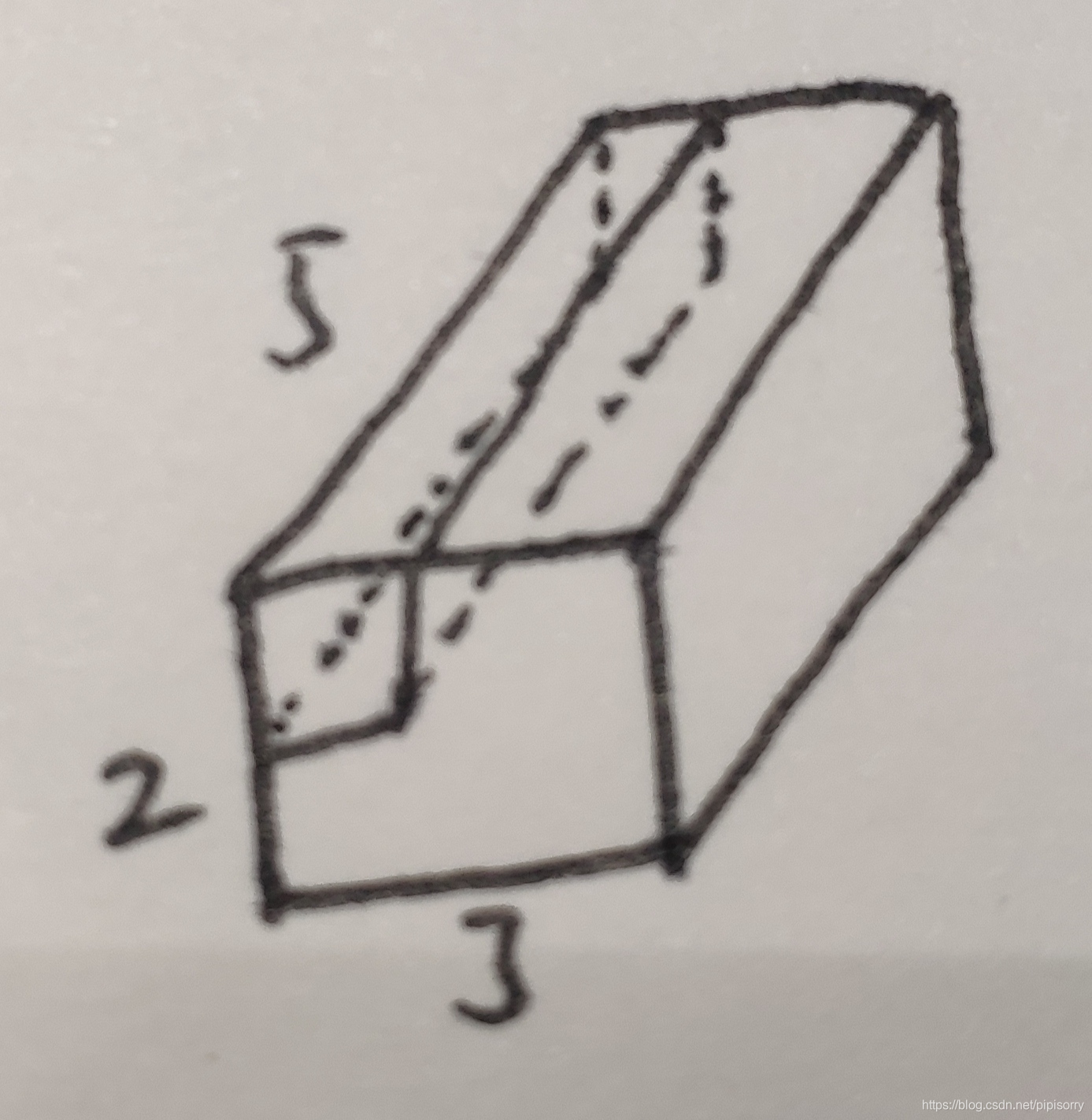
对于n维张量，如果dim=k，那就是对k维度进行softmax（这时其它维度取固定值时，维度k上的值加起来为1。）。比k更高维度的d(d<k)是不需要考虑的，直接去掉分析。
示例1：

t = torch.zeros([5,2,3])
t1 = torch.softmax(t, dim = 0)
t1：
tensor([[[0.2000, 0.2000, 0.2000],
         [0.2000, 0.2000, 0.2000]],
        [[0.2000, 0.2000, 0.2000],
         [0.2000, 0.2000, 0.2000]],
        [[0.2000, 0.2000, 0.2000],
         [0.2000, 0.2000, 0.2000]],
        [[0.2000, 0.2000, 0.2000],
         [0.2000, 0.2000, 0.2000]],
        [[0.2000, 0.2000, 0.2000],
         [0.2000, 0.2000, 0.2000]]])
t1[:,0,0]
tensor([0.2000, 0.2000, 0.2000, 0.2000, 0.2000])
sum(t1[:,0,0])
tensor(1.)

图的表示为（只对立方体中的k维度进行）：

示例2：如果有更高维度不用管
t = torch.zeros([4,5,2,3])
t1 = torch.softmax(t, dim = 1)
sum(t1[0,:,0,0])
tensor(1.)
示例3：

对2个维度同时进行softmax（即其它维度固定时，这2个维度的值加起来为1）。
t = torch.zeros([4,5,2,3])
# t1 = torch.softmax(t, dim = (1,2))， dim只能是数字，下面就是要模拟这个操作。
t1 = t.view(t.size(0), -1, t.size()[-1])
t2 = torch.softmax(t1, dim = 1).view(t.size())
t2[0,:,:,0].sum()
Out[14]: tensor(1.0000)
# sum(t2[0,:,:,0])
# Out[13]: tensor([0.5000, 0.5000])

[torch.nn.Softmax(dim=None)]

from: -柚子皮-

ref: [[Pytorch和Tensorflow对比（一）]：乘法、正则化]