07.Knowing When to Look

前言

本课程来自深度之眼《多模态》训练营,部分截图来自课程视频。
文章标题:Knowing When to Look: Adaptive Attention via A Visual Sentinel for Image Captioning

用于密集字幕的全卷积定位网络
作者:Jiasen Lu等
单位:弗吉尼亚理工大学
发表时间:2016 CVPR
Latex 公式编辑器

泛读

摘要

Attention-based neural encoder-decoder frameworks have been widely adopted for image captioning. Most methods force visual attention to be active for every generated word. However, the decoder likely requires little to no visual information from the image to predict non-visual words such as “the” and “of”. Other words that may seem visual can often be predicted reliably just from the language model e.g., “sign” after “behind a red stop” or “phone” following “talking on a cell”.
铺垫现有的问题是什么?
基于注意力的神经网络编码器-解码器框架已被广泛用于图像caption任务。大多数方法都强迫视觉注意力对每个生成的单词都处于激活状态。然而,解码器在预测 "the "和 "of "等非视觉单词时,可能几乎不需要来自图像的视觉信息。其他看似视觉性的单词往往可以通过语言模型可靠地预测出来,例如 "在红灯…的后面 "后的 "标志 "或 "手机通话 "后的 “电话”。

In this paper, we propose a novel adaptive attention model with a visual sentinel. At each time step, our model decides whether to attend to the image (and if so, to which regions) or to the visual sentinel. The model decides whether to attend to the image and where, in order to extract meaningful information for sequential word generation.
本文解决什么?
在本文中,我们提出了一种带有视觉哨点的新型自适应注意力模型。在每个时间步,我们的模型都会决定是关注图像(如果是,则关注哪些区域)还是视觉哨点。该模型会决定是否关注图像以及关注哪些区域,以便提取有意义的信息用于连续单词的生成。

We test our method on the COCO image captioning 2015 challenge dataset and Flickr30K. Our approach sets the new state-of-the-art by a significant margin.
效果如何?
我们在 COCO 2015 图像标题挑战数据集和 Flickr30K 上测试了我们的方法。我们的方法在很大程度上达到了SOTA。

Introduction

为图像自动生成字幕已经成为学术界和工业界的一个突出的跨学科研究问题。它可以帮助视力受损的用户,并使用户很容易地组织和浏览大量典型
的非结构化视觉数据。为了生成高质量的标题,模型需要从图像中结合细粒度的视觉线索。最近,现有研究是基于视觉注意的神经编码器-解码器模型,其中注意机制通常会生成一个空间地图,突出显示与每个生成的单词相关的图像区域。常见框架是注意力机制下的encoder-decoder(CNN+RNN)。

描述完现有的方法和模型后,对现有问题进行分析:
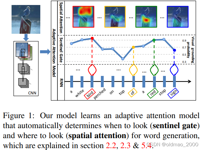
大多数用于图像配图和视觉问题回答的注意力模型在每个时间步都关注图像,而不管接下来将发出哪个单词。然而,并不是所有的文字都有相应的视觉信号。考虑图1中的示例,该图像显示了一个图像及其生成的标题“一
只白色的鸟栖息在红色停止标志上”单词“a”和“of”没有相应的规范视觉信号。此外,语言的相关性使视觉信号变得不必要,比如在生成单词“on”和“top”时,会生成单词“perched”,在生成单词“sign”时,会生成单词“a red stop。事实上,来自非视觉词的梯度可能会误导和降低视觉信号在指导标题生成过程中的整体有效性。
例如下图中单词bird,red对应的图片信号较高,而of,sign得分较少。这里的得分使用的metric是visual grounding(指代理解),主要是看给出的单词或短语对应图片区域的可信度的高低。
在这里插入图片描述
然后顺势提出本文的解决方案:
本文介绍了一种自适应注意力编码器-解码器框架,该框架可以自动决定何时依赖视觉信号,何时仅依赖语言模型。当然,当依赖于视觉信号时,模型也决定它应该关注哪里——哪个图像区域。首先提出了一种新的空间注意力模型来提取空间图像特征。然后,作为我们提出的自适应注意机制,我们引入了一个新的长短期记忆(LSTM)扩展,它产生了一个额外的“视觉哨兵”向量,而不是单一的隐藏状态。“视觉哨兵”是解码器内存的一个额外的潜在表示,为解码器提供了一个备用选项。我们进一步设计了一个新的前哨门,决定解码器希望从图像中获得多少新信息,而不是在生成下一个单词时依赖视觉哨兵。例如,如图1所示,我们的模型在生成单词“white”、“bird”、“red”和“stop”时学习更多地关注图像,在生成单词“top”、“of”和“sign”时更多地依赖视觉哨兵。

最后归纳全面的highlight:

  • 我们介绍了一种自适应编码器-解码器框架,它能自动决定何时查看图像,何时依靠语言模型生成下一个单词。(点题)
  • 我们首先提出了一种新的空间注意力模型,然后在此基础上设计出了带有 "视觉哨兵 "的新型自适应注意力模型。
  • 我们的模型在 COCO 和 Flickr30k 上的表现明显优于其他先进方法。
  • 我们对自适应注意力模型进行了广泛的分析,包括单词的视觉接地概率和生成的注意力地图的弱监督定位。

小结

1.引入了Spatial Attention的模型;(图像和文本之间的attention关联依旧很重要)
2.提出了Adaptive Attention,让网络自适应的去决定依靠视觉信息或语言模型:哨兵监控

精讲

方法

related work这节往后放了。

Encoder-Decoder框架 for Image Captioning

给定一个图像和相应的标题,先给出Encoder-Decoder框架的目标函数:
θ ∗ = arg max ⁡ θ ∑ I , y log ⁡ p ( y ∣ I ; θ ) \theta^*=\argmax_{\theta}\sum_{I,y}\log p(y|I;\theta) θ=θargmaxI,ylogp(yI;θ)
其中 θ \theta θ是模型的参数, I I I为图像, y = { y 1 , ⋯   , y t } y=\{y_1,\cdots,y_t\} y={y1,,yt}caption得到的序列。
利用链式法则,联合概率分布的对数似然可以分解为有序条件:
log ⁡ p ( y ) = ∑ t = 1 T log ⁡ p ( y t ∣ y 1 , ⋯   , y t − 1 , I ) \log p(y)=\sum_{t=1}^T\log p(y_t|y_1,\cdots,y_{t-1},I) logp(y)=t=1Tlogp(yty1,,yt1,I)
为了方便,我们放弃了对模型参数的依赖。
在编码器-解码器框架中,使用循环神经网络(RNN),每个条件概率被建模为:
log ⁡ p ( y t ∣ y 1 , ⋯   , y t − 1 , I ) = f ( h t , c t ) (3) \log p(y_t|y_1,\cdots,y_{t-1},I)=f(h_t,c_t)\tag 3 logp(yty1,,yt1,I)=f(ht,ct)(3)
其中 f f f是非线性函数, c t c_t ct是在 t t t时间步从图像 I I I中提取到的上下文向量。 h t h_t ht是RNN在 t t t时间步的隐藏层。本文RNN选用的是LSTM,其隐藏层公式为:
h t = LSTM ( x t , h t − 1 , m t − 1 ) h_t=\text{LSTM}(x_t,h_{t-1},m_{t-1}) ht=LSTM(xt,ht1,mt1)
x t x_t xt是输入向量, m t − 1 m_{t-1} mt1 t − 1 t-1 t1时间步的存储记忆单元。
通常,上下文向量 c t c_t ct是神经编码器-解码器框架中的一个重要因素,它为caption生成提供了视觉证据。
这些建模上下文向量的不同方法分为两类:
1.原版编码器-解码器框架
原版框架中, c t c_t ct只与编码器有关,一般编码器使用CNN模型。CNN吃进图像 I I I,最后从全连接层得到图片的全局特征。在解码过程中, c t c_t ct相当于常量,不变,不会依赖于编码器的隐藏层。

2.基于注意力的编码器-解码器框架。
在这种框架中, c t c_t ct与编码和解码器都有关系。在解码过程的第 t t t时间步,解码器会根据特定的图片区域,以及对应的区域特征 c t c_t ct来进行计算。已有文献已证明该方法效果很不错。

本文对计算 c t c_t ct提出了spatial attention model,还对齐进行了扩展,升级为: adaptive attention model

Spatial Attention Model

先给出空间注意力模型计算上下文特征 c t c_t ct的公式:
c t = g ( V , h t ) c_t=g(V,h_t) ct=g(V,ht)
其中 g g g是注意力函数;
V = [ v 1 , ⋯   , v k ] , v i ∈ R d V=[v_1,\cdots,v_k],v_i\in \mathcal{R}^d V=[v1,,vk],viRd是图片空间特征,每一个特征都是对应于图像的一部分的 d d d维表示;
h t h_t ht是RNN在 t t t时刻的隐藏层。
给定图片空间特征 V ∈ R d × k V\in \mathcal{R}^{d\times k} VRd×k,LSTM的隐藏层 h t ∈ R d h_t\in\mathcal{R}^d htRd,将它们丢进单层带softmax的神经网络,可获得生成图像 k k k个区域上的注意力分布:
z t = w h T tanh ⁡ ( W v V + ( W g h t ) 1 T ) (6) z_t=w^T_h\tanh(W_vV+(W_gh_t)\mathbf{1}^T)\tag 6 zt=whTtanh(WvV+(Wght)1T)(6)
α t = softmax ( z t ) (7) \alpha_t=\text{softmax}(z_t)\tag 7 αt=softmax(zt)(7)

这里的 1 \mathbf{1} 1应该显示为:在这里插入图片描述
但是markdown不支持\mathbb{1}显示。
1 ∈ R k \mathbf{1}\in\mathcal{R}^k 1Rk是一个全1的向量
W v , W g ∈ R k × d W_v,W_g\in\mathcal{R}^{k\times d} Wv,WgRk×d w h ∈ R k w_h\in\mathcal{R}^k whRk都是需要训练的参数。
α t ∈ R k \alpha_t\in \mathcal{R}^k αtRk图片空间特征 V V V的注意力权重。
根据注意力分布,上下文向量 c t c_t ct的公式为:
c t = ∑ i = 1 k α t i v t i c_t=\sum_{i=1}^k\alpha_{ti}v_{ti} ct=i=1kαtivti
c t , h t c_t,h_t ct,ht将合起来预测公式3中的下一个词 y t + 1 y_{t+1} yt+1

在这里插入图片描述
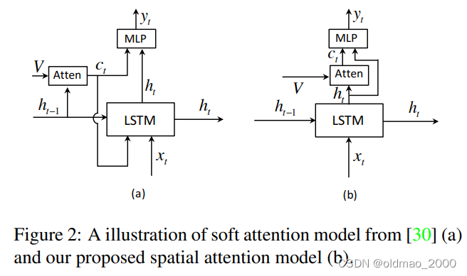
图2中提到的文献30,就是前面第4篇带读的Show, Attend and Tell,这里作者用其为对比,说明本文使用了隐藏层 h t h_t ht来分析要关注图片的区域(也就是生成 c t c_t ct),然后结合这两个信息源来预测下一个单词。我们的动机源于残差网络。生成的上下文向量 c t c_t ct可以看作是当前隐藏状态 h t h_t ht的剩余视觉信息,减少了当前隐藏状态的不确定性或补充了下一个词预测的信息量。我们还从经验上发现,我们的空间注意力模型表现得更好(具体看实验)。

Adaptive Attention Model

虽然基于空间注意力的解码器已被证明对图像caption是有效的,但它们不能确定何时依赖视觉信号,何时依赖语言模型。本文受Merity等[19]的启发,我们引入了一个新概念:“视觉哨兵”,这是解码器已经知道的东西的潜在表示。通过“视觉哨兵”,我们扩展了我们的空间注意力模型,并提出了一个自适应模型,能够确定它是否需要关注图像来预测下一个单词。
然后给出视觉哨兵的定义:
解码器的内存中存储着长期和短期的视觉和语言信息。我们的模型学会了从中提取一个新的组成部分,当模型选择不关注图像时,它就可以利用这个新的组成部分。这一新部分被称为视觉哨兵。而决定是关注图像还是视觉哨兵的门就是哨兵门。当解码器是LSTM时,我们会考虑其存储单元中保存的信息。扩展后的LSTM获取视觉哨兵向量 s t s_t st的公式如下:
g t = σ ( W x x t + W h h t − 1 ) s t = g t ⊙ tanh ⁡ ( m t ) g_t=\sigma(W_xx_t+W_hh_{t-1})\\ s_t=g_t\odot\tanh(m_t) gt=σ(Wxxt+Whht1)st=gttanh(mt)
其中 W x , W h W_x,W_h Wx,Wh是要学习的参数;
x t x_t xt是LSTM在 t t t时间步的输入;
g t g_t gt是记忆存储单元 m t m_t mt的门控;
⊙ \odot 表示元素点乘;
σ \sigma σ表示逻辑激活函数。
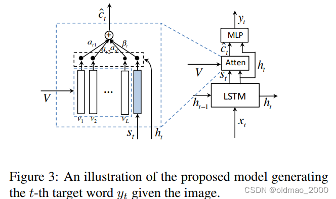
根据视觉哨兵,本文提出了自适应注意力模型来计算上下文向量。如下图所示:
在这里插入图片描述
上下文向量为 c ^ t \hat c_t c^t,由空间参与图像特征(即空间注意模型的上下文向量)和视觉哨兵向量共同计算得来,该向量可权衡网络从图像中考虑的新信息与它在解码器内存中已经知道的信息(即视觉哨兵)。其公式如下:
c ^ t = β t s t + ( 1 − β t ) c t \hat c_t=\beta_ts_t+(1-\beta_t)c_t c^t=βtst+(1βt)ct
其中, β t \beta_t βt t t t时刻的哨兵门控,与其他门控取值范围一样: [ 0 , 1 ] [0,1] [0,1]。1表示在生成下一个单词时仅使用视觉哨兵信息(公式的后面一项为0),0则表示仅使用空间图像信息(公式的前面一项为0)。
为计算 β t \beta_t βt,文中定义了空间注意力组件,就是上面公式6中的 z z z,它表示网络对于哨兵的关注程度,因此公式7可以写为:
α ^ t = softmax ( [ z t ; w h T tanh ⁡ ( W s s t + ( W g h t ) ) ] ) \hat\alpha_t=\text{softmax}([z_t;w_h^T\tanh(Wss_t+(W_gh_t))]) α^t=softmax([zt;whTtanh(Wsst+(Wght))])
这里的 [ ⋅ ; ⋅ ] [\cdot ;\cdot] [;]表示concat操作,spatial attention部分k个区域的attention分布 α t \alpha_t αt也被扩展成了 α ^ t \hat\alpha_t α^t,做法是在 z t z_t zt后面拼接上上面公式的那一坨;
W s , W g W_s,W_g Ws,Wg是权重参数, W g W_g Wg与公式6中的notation一致,含义也相同;
α ^ t ∈ R k + 1 \hat\alpha_t\in\mathcal{R}^{k+1} α^tRk+1是视觉哨兵(也可以说是空间图片特征,二者是此消彼长的关系)向量的注意力分布。
这里使用 α ^ t \hat\alpha_t α^t向量的最后一个元素表示门控值: β t = α t [ k + 1 ] \beta_t=\alpha_t[k+1] βt=αt[k+1]
t t t时刻,从词表中抽取某个词的概率可表示为:
p t = softmax ( W p ( c ^ t + h t ) ) p_t=\text{softmax}(W_p(\hat c_t+h_t)) pt=softmax(Wp(c^t+ht))
W p W_p Wp是待学习参数。
这个公式表明模型在生成词的时候会自适应图片是哨兵之间的注意力。由于哨兵向量在每个时间步都更新,因此整个框架又称为自适应编码解码图片captioning框架。

Implementation Details

Encoder-CNN

图像选择了ResNet的最后一层卷积层的特征来表示图像,维度是 2048 × 7 × 7 2048\times7\times7 2048×7×7,全局图像特征则是局部特征的平均。局部图像特征需要经过转换,CNN特征的 k k k个网格区域表示为 A = { a 1 , ⋯   , a k } , a i ∈ R 2048 A=\{a_1,\cdots,a_k\},a_i\in\mathcal{R}^{2048} A={a1,,ak},aiR2048,全局图片特征为:
a g = 1 k ∑ i = 1 k a i a^g=\cfrac{1}{k}\sum_{i=1}^ka_i ag=k1i=1kai
为了建模方便,这里使用了单层整流激活函数将图片特征向量投影到 d d d维的新向量:
v i = ReLU ( W a a i ) v g = ReLU ( W b a g ) v_i=\text{ReLU}(W_aa_i)\\ v^g=\text{ReLU}(W_ba^g) vi=ReLU(Waai)vg=ReLU(Wbag)
W a , W g W_a,W_g Wa,Wg是权重参数,投影后的向量可写为: V = [ v 1 , ⋯   , v k ] V=[v_1,\cdots,v_k] V=[v1,,vk]

Decoder-RNN

将词向量和全局图片特征进行concat后作为LSTM的输入( x t = [ w t ; v g ] x_t=[w_t;v^g] xt=[wt;vg]),然后用单层神经网络将视觉哨兵 s t s_t st和LSTM输出向量 h t h_t ht投影到 d d d维空间。

Training details

使用单层LSTM,隐藏层大小为512,优化器用的Adam,LSTM学习率为 5 e − 4 5e-4 5e4,CNN学习率为 1 e − 5 1e-5 1e5,momentum和权重衰减分别为0.8和0.999。
先对CNN微调20个epoch,然后把batchsize设置为80,再训练50个epoch,如果训练过程中CIDEr在6个epoch内没有变化则采取early stopping机制提前结束训练。
模型在单张泰坦X GPU上训练30小时就完成既定目标。

Related Work

很多文章把本该放在Introduction后面的这个小节放到介绍自己的框架或者方法后面。
原文大概介绍了图形生成文本的重要作用,然后总结目前生成文本有两种方法:基于模板和基于神经网络。
然后分小节分别进行介绍,基于模板的研究不展开。
基于神经的方法受到机器翻译中序列到序列编码器-解码器框架成功的启发。其观点是图像字幕类似于将图像翻译为文本。
最近,注意机制被引入到图像字幕的编码器-解码器神经框架中。这块花的笔墨较重。
当然最后不免要吹嘘一下自己的工作:
To the best of our knowledge, ours is the first work to reason about when a model should attend to an image when generating a sequence of words.

实验

在这里插入图片描述
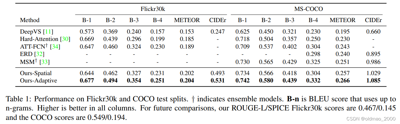
表1给出了不同方法在在Flickr30k和MSCOCO的测试集上的运行结果,Metric包括BLUE、METEOR和CIDEr,分数都是越高越好,可以看到最高分都在Adaptive那行,当然Spatial就很厉害了。

在这里插入图片描述
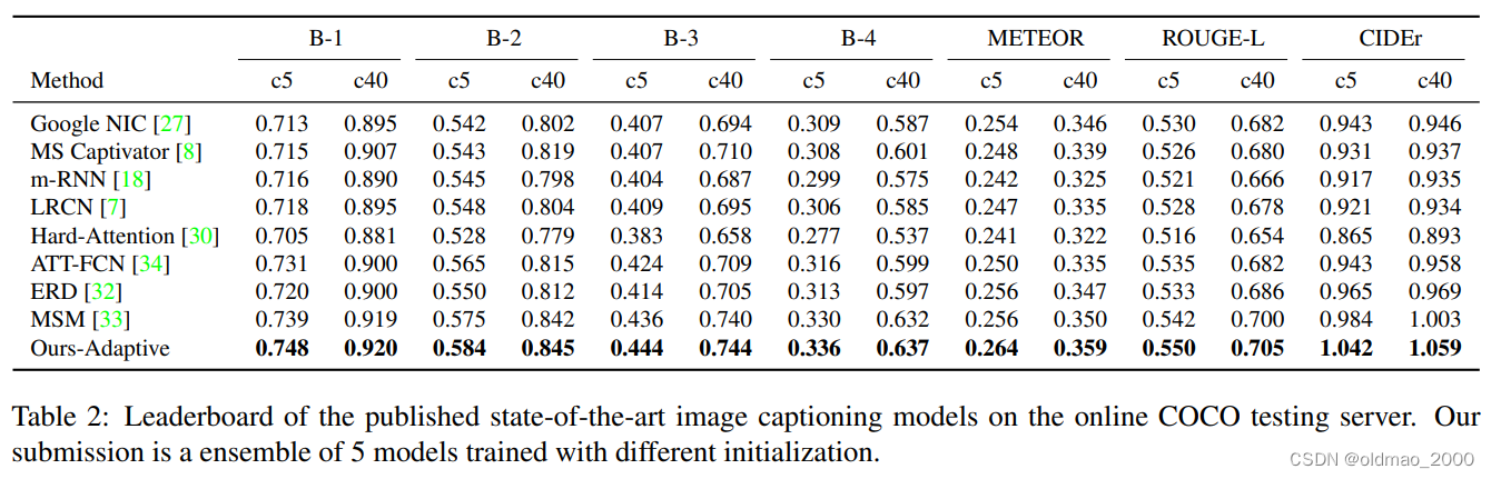
表2直接给出了公共测试服务器上的对比结果,当然本文使用了ensemble。

在这里插入图片描述
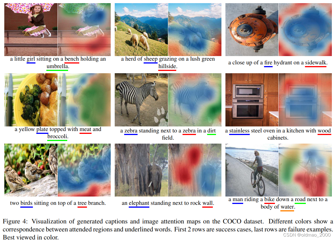
图4显示了生成的标题和标题中特定单词的空间注意图。前两列是成功的例子,最后一列是失败的例子。我们看到,我们的模型学习的对齐方式与人类直觉强烈一致。请注意,即使在模型产生不准确的标题的情况下,我
们看到我们的模型确实看到了图像中的合理区域,只不过它似乎无法计数或识别纹理(或材质)和细粒度类别。这里作者暗示未来可以针对这里进行改进,如果CNN能够更加强,对应的效果自然会更加好。
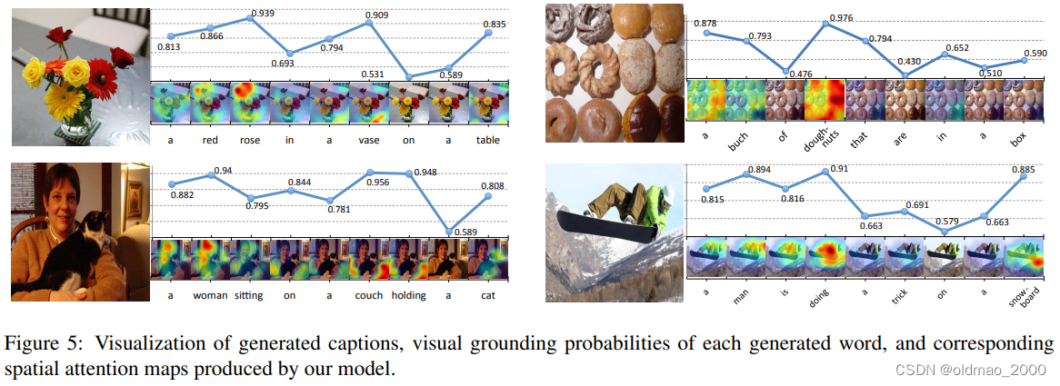
在这里插入图片描述
图5主要是哨兵门概率 1 − β 1−β 1β的可视化,对于视觉词,模型给出的概率较大,即更倾向于关注图像特征 c t c_t ct,对于非视觉词的概率则比较小(例如:“the”, “of”, “to”等定冠词、介词)。同时,同一个词在不同的上下文中的概率也是不一样的。如"a",在一开始的概率较高,因为开始时没有任何的语义信息可以依赖、以及需要确定单复数。

在这里插入图片描述
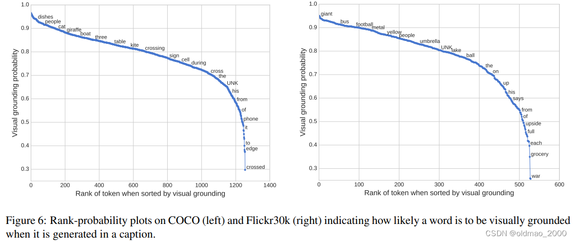
上图将词表中每个单词的 visual grounding probability用点图的方式画出来。每个单词都是计算了生成概率的平均值。从图中可以看到,模型对于实体词:“dishes”, “people”, “cat”,“boat”;描述词(形容词)“giant”, “metal”, “yellow”;数词 “three”等会给比较大视觉注意力,对于定冠词、介词“the”,“of”, “to”等会给比较少,而对于抽象表示词“crossing”, “during” 等会给出介于前面两类之间的视觉注意力。文章还特别指出模型的视觉注意力分布并不依赖于任何语义或者额外的领域知识,都是自动学习的。

有一些例外,例如“phone”获得的视觉注意力较低,因为它在训练数据中通常是以“cell phone”的形式出现,由于“cell”获得的视觉注意力较高,且二者同时出现频率较高(强相关),也就解释了“phone”获得较低视觉注意力的原因。

在这里插入图片描述

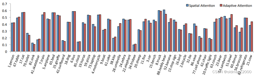
上图显示了两个模型(spatial和adaptive attention)在COCO数据集中出现最频繁的(top 45)词的定位准确性。对于一些体积较小的物体(“sink”, “surfboard”, “clock” and “frisbee”),其准确率是比较低的,这是因为attention map是从7x7的featuremap中直接放大的,而7x7的feature map并不能很好地包含这些小物体的信息。较大物体反之。(“cat”, “bed”, “bus”, “truck”)

结论

很短,没有讨论和展望。
在本文中,我们提出了一种新的自适应注意力编码器-解码器框架,该框架为解码器提供了一个回退选项。我们进一步引入了一个新的LSTM扩展,它产生了一个额外的“视觉哨兵”。
我们的模型在图像字幕的标准基准上实现了最先进的性能。我们进行广泛的注意评估来分析我们的适应性注意。虽然我们的模型是在图像caption任务上进行评估的,但它也可以应用在其他领域。

Quickstart Note The data files used in the quickstart guide are updated from time to time, which means that the adjusted close changes and with it the close (and the other components). That means that the actual output may be different to what was put in the documentation at the time of writing. Using the platform Let’s run through a series of examples (from almost an empty one to a fully fledged strategy) but not without before roughly explaining 2 basic concepts when working with backtrader Lines Data Feeds, Indicators and Strategies have lines. A line is a succession of points that when joined together form this line. When talking about the markets, a Data Feed has usually the following set of points per day: Open, High, Low, Close, Volume, OpenInterest The series of “Open”s along time is a Line. And therefore a Data Feed has usually 6 lines. If we also consider “DateTime” (which is the actual reference for a single point), we could count 7 lines. Index 0 Approach When accessing the values in a line, the current value is accessed with index: 0 And the “last” output value is accessed with -1. This in line with Python conventions for iterables (and a line can be iterated and is therefore an iterable) where index -1 is used to access the “last” item of the iterable/array. In our case is the last output value what’s getting accessed. As such and being index 0 right after -1, it is used to access the current moment in line. With that in mind and if we imagine a Strategy featuring a Simple Moving average created during initialization: self.sma = SimpleMovingAverage(.....) The easiest and simplest way to access the current value of this moving average: av = self.sma[0] There is no need to know how many bars/minutes/days/months have been processed, because “0” uniquely identifies the current instant. Following pythonic tradition, the “last” output value is accessed using -1: previous_value = self.sma[-1] Of course earlier output values can be accessed with -2, -3, … From 0 to 100: the samples Basic Setup Let’s get running. from __future__ import (absolute_import, division, print_function, unicode_literals) import backtrader as bt if __name__ == '__main__': cerebro = bt.Cerebro() print('Starting Portfolio Value: %.2f' % cerebro.broker.getvalue()) cerebro.run() print('Final Portfolio Value: %.2f' % cerebro.broker.getvalue()) After the execution the output is: Starting Portfolio Value: 10000.00 Final Portfolio Value: 10000.00 In this example: backtrader was imported The Cerebro engine was instantiated The resulting cerebro instance was told to run (loop over data) And the resulting outcome was printed out Although it doesn’t seem much, let’s point out something explicitly shown: The Cerebro engine has created a broker instance in the background The instance already has some cash to start with This behind the scenes broker instantiation is a constant trait in the platform to simplify the life of the user. If no broker is set by the user, a default one is put in place. And 10K monetary units is a usual value with some brokers to begin with. Setting the Cash In the world of finance, for sure only “losers” start with 10k. Let’s change the cash and run the example again. from __future__ import (absolute_import, division, print_function, unicode_literals) import backtrader as bt if __name__ == '__main__': cerebro = bt.Cerebro() cerebro.broker.setcash(100000.0) print('Starting Portfolio Value: %.2f' % cerebro.broker.getvalue()) cerebro.run() print('Final Portfolio Value: %.2f' % cerebro.broker.getvalue()) After the execution the output is: Starting Portfolio Value: 1000000.00 Final Portfolio Value: 1000000.00 Mission accomplished. Let’s move to tempestuous waters. Adding a Data Feed Having cash is fun, but the purpose behind all this is to let an automated strategy multiply the cash without moving a finger by operating on an asset which we see as a Data Feed Ergo … No Data Feed -> No Fun. Let’s add one to the ever growing example. from __future__ import (absolute_import, division, print_function, unicode_literals) import datetime # For datetime objects import os.path # To manage paths import sys # To find out the script name (in argv[0]) # Import the backtrader platform import backtrader as bt if __name__ == '__main__': # Create a cerebro entity cerebro = bt.Cerebro() # Datas are in a subfolder of the samples. Need to find where the script is # because it could have been called from anywhere modpath = os.path.dirname(os.path.abspath(sys.argv[0])) datapath = os.path.join(modpath, '../../datas/orcl-1995-2014.txt') # Create a Data Feed data = bt.feeds.YahooFinanceCSVData( dataname=datapath, # Do not pass values before this date fromdate=datetime.datetime(2000, 1, 1), # Do not pass values after this date todate=datetime.datetime(2000, 12, 31), reverse=False) # Add the Data Feed to Cerebro cerebro.adddata(data) # Set our desired cash start cerebro.broker.setcash(100000.0) # Print out the starting conditions print('Starting Portfolio Value: %.2f' % cerebro.broker.getvalue()) # Run over everything cerebro.run() # Print out the final result print('Final Portfolio Value: %.2f' % cerebro.broker.getvalue()) After the execution the output is: Starting Portfolio Value: 1000000.00 Final Portfolio Value: 1000000.00 The amount of boilerplate has grown slightly, because we added: Finding out where our example script is to be able to locate the sample Data Feed file Having datetime objects to filter on which data from the Data Feed we will be operating Aside from that, the Data Feed is created and added to cerebro. The output has not changed and it would be a miracle if it had. Note Yahoo Online sends the CSV data in date descending order, which is not the standard convention. The reversed=True prameter takes into account that the CSV data in the file has already been reversed and has the standard expected date ascending order. Our First Strategy The cash is in the broker and the Data Feed is there. It seems like risky business is just around the corner. Let’s put a Strategy into the equation and print the “Close” price of each day (bar). DataSeries (the underlying class in Data Feeds) objects have aliases to access the well known OHLC (Open High Low Close) daily values. This should ease up the creation of our printing logic. from __future__ import (absolute_import, division, print_function, unicode_literals) import datetime # For datetime objects import os.path # To manage paths import sys # To find out the script name (in argv[0]) # Import the backtrader platform import backtrader as bt # Create a Stratey class TestStrategy(bt.Strategy): def log(self, txt, dt=None): ''' Logging function for this strategy''' dt = dt or self.datas[0].datetime.date(0) print('%s, %s' % (dt.isoformat(), txt)) def __init__(self): # Keep a reference to the "close" line in the data[0] dataseries self.dataclose = self.datas[0].close def next(self): # Simply log the closing price of the series from the reference self.log('Close, %.2f' % self.dataclose[0]) if __name__ == '__main__': # Create a cerebro entity cerebro = bt.Cerebro() # Add a strategy cerebro.addstrategy(TestStrategy) # Datas are in a subfolder of the samples. Need to find where the script is # because it could have been called from anywhere modpath = os.path.dirname(os.path.abspath(sys.argv[0])) datapath = os.path.join(modpath, '../../datas/orcl-1995-2014.txt') # Create a Data Feed data = bt.feeds.YahooFinanceCSVData( dataname=datapath, # Do not pass values before this date fromdate=datetime.datetime(2000, 1, 1), # Do not pass values before this date todate=datetime.datetime(2000, 12, 31), # Do not pass values after this date reverse=False) # Add the Data Feed to Cerebro cerebro.adddata(data) # Set our desired cash start cerebro.broker.setcash(100000.0) # Print out the starting conditions print('Starting Portfolio Value: %.2f' % cerebro.broker.getvalue()) # Run over everything cerebro.run() # Print out the final result print('Final Portfolio Value: %.2f' % cerebro.broker.getvalue()) After the execution the output is: Starting Portfolio Value: 100000.00 2000-01-03T00:00:00, Close, 27.85 2000-01-04T00:00:00, Close, 25.39 2000-01-05T00:00:00, Close, 24.05 ... ... ... 2000-12-26T00:00:00, Close, 29.17 2000-12-27T00:00:00, Close, 28.94 2000-12-28T00:00:00, Close, 29.29 2000-12-29T00:00:00, Close, 27.41 Final Portfolio Value: 100000.00 Someone said the stockmarket was risky business, but it doesn’t seem so. Let’s explain some of the magic: Upon init being called the strategy already has a list of datas that are present in the platform This is a standard Python list and datas can be accessed in the order they were inserted. The first data in the list self.datas[0] is the default data for trading operations and to keep all strategy elements synchronized (it’s the system clock) self.dataclose = self.datas[0].close keeps a reference to the close line. Only one level of indirection is later needed to access the close values. The strategy next method will be called on each bar of the system clock (self.datas[0]). This is true until other things come into play like indicators, which need some bars to start producing an output. More on that later. Adding some Logic to the Strategy Let’s try some crazy idea we had by looking at some charts If the price has been falling 3 sessions in a row … BUY BUY BUY!!! from __future__ import (absolute_import, division, print_function, unicode_literals) import datetime # For datetime objects import os.path # To manage paths import sys # To find out the script name (in argv[0]) # Import the backtrader platform import backtrader as bt # Create a Stratey class TestStrategy(bt.Strategy): def log(self, txt, dt=None): ''' Logging function fot this strategy''' dt = dt or self.datas[0].datetime.date(0) print('%s, %s' % (dt.isoformat(), txt)) def __init__(self): # Keep a reference to the "close" line in the data[0] dataseries self.dataclose = self.datas[0].close def next(self): # Simply log the closing price of the series from the reference self.log('Close, %.2f' % self.dataclose[0]) if self.dataclose[0] < self.dataclose[-1]: # current close less than previous close if self.dataclose[-1] < self.dataclose[-2]: # previous close less than the previous close # BUY, BUY, BUY!!! (with all possible default parameters) self.log('BUY CREATE, %.2f' % self.dataclose[0]) self.buy() if __name__ == '__main__': # Create a cerebro entity cerebro = bt.Cerebro() # Add a strategy cerebro.addstrategy(TestStrategy) # Datas are in a subfolder of the samples. Need to find where the script is # because it could have been called from anywhere modpath = os.path.dirname(os.path.abspath(sys.argv[0])) datapath = os.path.join(modpath, '../../datas/orcl-1995-2014.txt') # Create a Data Feed data = bt.feeds.YahooFinanceCSVData( dataname=datapath, # Do not pass values before this date fromdate=datetime.datetime(2000, 1, 1), # Do not pass values before this date todate=datetime.datetime(2000, 12, 31), # Do not pass values after this date reverse=False) # Add the Data Feed to Cerebro cerebro.adddata(data) # Set our desired cash start cerebro.broker.setcash(100000.0) # Print out the starting conditions print('Starting Portfolio Value: %.2f' % cerebro.broker.getvalue()) # Run over everything cerebro.run() # Print out the final result print('Final Portfolio Value: %.2f' % cerebro.broker.getvalue()) After the execution the output is: Starting Portfolio Value: 100000.00 2000-01-03, Close, 27.85 2000-01-04, Close, 25.39 2000-01-05, Close, 24.05 2000-01-05, BUY CREATE, 24.05 2000-01-06, Close, 22.63 2000-01-06, BUY CREATE, 22.63 2000-01-07, Close, 24.37 ... ... ... 2000-12-20, BUY CREATE, 26.88 2000-12-21, Close, 27.82 2000-12-22, Close, 30.06 2000-12-26, Close, 29.17 2000-12-27, Close, 28.94 2000-12-27, BUY CREATE, 28.94 2000-12-28, Close, 29.29 2000-12-29, Close, 27.41 Final Portfolio Value: 99725.08 Several “BUY” creation orders were issued, our porftolio value was decremented. A couple of important things are clearly missing. The order was created but it is unknown if it was executed, when and at what price. The next example will build upon that by listening to notifications of order status. The curious reader may ask how many shares are being bought, what asset is being bought and how are orders being executed. Where possible (and in this case it is) the platform fills in the gaps: self.datas[0] (the main data aka system clock) is the target asset if no other one is specified The stake is provided behind the scenes by a position sizer which uses a fixed stake, being the default “1”. It will be modified in a later example The order is executed “At Market”. The broker (shown in previous examples) executes this using the opening price of the next bar, because that’s the 1st tick after the current under examination bar. The order is executed so far without any commission (more on that later) Do not only buy … but SELL After knowing how to enter the market (long), an “exit concept” is needed and also understanding whether the strategy is in the market. Luckily a Strategy object offers access to a position attribute for the default data feed Methods buy and sell return the created (not yet executed) order Changes in orders’ status will be notified to the strategy via a notify method The “exit concept” will be an easy one: Exit after 5 bars (on the 6th bar) have elapsed for good or for worse Please notice that there is no “time” or “timeframe” implied: number of bars. The bars can represent 1 minute, 1 hour, 1 day, 1 week or any other time period. Although we know the data source is a daily one, the strategy makes no assumption about that. Additionally and to simplify: Do only allow a Buy order if not yet in the market Note The next method gets no “bar index” passed and therefore it seems obscure how to understand when 5 bars may have elapsed, but this has been modeled in pythonic way: call len on an object and it will tell you the length of its lines. Just write down (save in a variable) at which length in an operation took place and see if the current length is 5 bars away. from __future__ import (absolute_import, division, print_function, unicode_literals) import datetime # For datetime objects import os.path # To manage paths import sys # To find out the script name (in argv[0]) # Import the backtrader platform import backtrader as bt # Create a Stratey class TestStrategy(bt.Strategy): def log(self, txt, dt=None): ''' Logging function fot this strategy''' dt = dt or self.datas[0].datetime.date(0) print('%s, %s' % (dt.isoformat(), txt)) def __init__(self): # Keep a reference to the "close" line in the data[0] dataseries self.dataclose = self.datas[0].close # To keep track of pending orders self.order = None def notify_order(self, order): if order.status in [order.Submitted, order.Accepted]: # Buy/Sell order submitted/accepted to/by broker - Nothing to do return # Check if an order has been completed # Attention: broker could reject order if not enough cash if order.status in [order.Completed]: if order.isbuy(): self.log('BUY EXECUTED, %.2f' % order.executed.price) elif order.issell(): self.log('SELL EXECUTED, %.2f' % order.executed.price) self.bar_executed = len(self) elif order.status in [order.Canceled, order.Margin, order.Rejected]: self.log('Order Canceled/Margin/Rejected') # Write down: no pending order self.order = None def next(self): # Simply log the closing price of the series from the reference self.log('Close, %.2f' % self.dataclose[0]) # Check if an order is pending ... if yes, we cannot send a 2nd one if self.order: return # Check if we are in the market if not self.position: # Not yet ... we MIGHT BUY if ... if self.dataclose[0] < self.dataclose[-1]: # current close less than previous close if self.dataclose[-1] < self.dataclose[-2]: # previous close less than the previous close # BUY, BUY, BUY!!! (with default parameters) self.log('BUY CREATE, %.2f' % self.dataclose[0]) # Keep track of the created order to avoid a 2nd order self.order = self.buy() else: # Already in the market ... we might sell if len(self) >= (self.bar_executed + 5): # SELL, SELL, SELL!!! (with all possible default parameters) self.log('SELL CREATE, %.2f' % self.dataclose[0]) # Keep track of the created order to avoid a 2nd order self.order = self.sell() if __name__ == '__main__': # Create a cerebro entity cerebro = bt.Cerebro() # Add a strategy cerebro.addstrategy(TestStrategy) # Datas are in a subfolder of the samples. Need to find where the script is # because it could have been called from anywhere modpath = os.path.dirname(os.path.abspath(sys.argv[0])) datapath = os.path.join(modpath, '../../datas/orcl-1995-2014.txt') # Create a Data Feed data = bt.feeds.YahooFinanceCSVData( dataname=datapath, # Do not pass values before this date fromdate=datetime.datetime(2000, 1, 1), # Do not pass values before this date todate=datetime.datetime(2000, 12, 31), # Do not pass values after this date reverse=False) # Add the Data Feed to Cerebro cerebro.adddata(data) # Set our desired cash start cerebro.broker.setcash(100000.0) # Print out the starting conditions print('Starting Portfolio Value: %.2f' % cerebro.broker.getvalue()) # Run over everything cerebro.run() # Print out the final result print('Final Portfolio Value: %.2f' % cerebro.broker.getvalue()) After the execution the output is: Starting Portfolio Value: 100000.00 2000-01-03T00:00:00, Close, 27.85 2000-01-04T00:00:00, Close, 25.39 2000-01-05T00:00:00, Close, 24.05 2000-01-05T00:00:00, BUY CREATE, 24.05 2000-01-06T00:00:00, BUY EXECUTED, 23.61 2000-01-06T00:00:00, Close, 22.63 2000-01-07T00:00:00, Close, 24.37 2000-01-10T00:00:00, Close, 27.29 2000-01-11T00:00:00, Close, 26.49 2000-01-12T00:00:00, Close, 24.90 2000-01-13T00:00:00, Close, 24.77 2000-01-13T00:00:00, SELL CREATE, 24.77 2000-01-14T00:00:00, SELL EXECUTED, 25.70 2000-01-14T00:00:00, Close, 25.18 ... ... ... 2000-12-15T00:00:00, SELL CREATE, 26.93 2000-12-18T00:00:00, SELL EXECUTED, 28.29 2000-12-18T00:00:00, Close, 30.18 2000-12-19T00:00:00, Close, 28.88 2000-12-20T00:00:00, Close, 26.88 2000-12-20T00:00:00, BUY CREATE, 26.88 2000-12-21T00:00:00, BUY EXECUTED, 26.23 2000-12-21T00:00:00, Close, 27.82 2000-12-22T00:00:00, Close, 30.06 2000-12-26T00:00:00, Close, 29.17 2000-12-27T00:00:00, Close, 28.94 2000-12-28T00:00:00, Close, 29.29 2000-12-29T00:00:00, Close, 27.41 2000-12-29T00:00:00, SELL CREATE, 27.41 Final Portfolio Value: 100018.53 Blistering Barnacles!!! The system made money … something must be wrong The broker says: Show me the money! And the money is called “commission”. Let’s add a reasonable 0.1% commision rate per operation (both for buying and selling … yes the broker is avid …) A single line will suffice for it: # 0.1% ... divide by 100 to remove the % cerebro.broker.setcommission(commission=0.001) Being experienced with the platform we want to see the profit or loss after a buy/sell cycle, with and without commission. from __future__ import (absolute_import, division, print_function, unicode_literals) import datetime # For datetime objects import os.path # To manage paths import sys # To find out the script name (in argv[0]) # Import the backtrader platform import backtrader as bt # Create a Stratey class TestStrategy(bt.Strategy): def log(self, txt, dt=None): ''' Logging function fot this strategy''' dt = dt or self.datas[0].datetime.date(0) print('%s, %s' % (dt.isoformat(), txt)) def __init__(self): # Keep a reference to the "close" line in the data[0] dataseries self.dataclose = self.datas[0].close # To keep track of pending orders and buy price/commission self.order = None self.buyprice = None self.buycomm = None def notify_order(self, order): if order.status in [order.Submitted, order.Accepted]: # Buy/Sell order submitted/accepted to/by broker - Nothing to do return # Check if an order has been completed # Attention: broker could reject order if not enough cash if order.status in [order.Completed]: if order.isbuy(): self.log( 'BUY EXECUTED, Price: %.2f, Cost: %.2f, Comm %.2f' % (order.executed.price, order.executed.value, order.executed.comm)) self.buyprice = order.executed.price self.buycomm = order.executed.comm else: # Sell self.log('SELL EXECUTED, Price: %.2f, Cost: %.2f, Comm %.2f' % (order.executed.price, order.executed.value, order.executed.comm)) self.bar_executed = len(self) elif order.status in [order.Canceled, order.Margin, order.Rejected]: self.log('Order Canceled/Margin/Rejected') self.order = None def notify_trade(self, trade): if not trade.isclosed: return self.log('OPERATION PROFIT, GROSS %.2f, NET %.2f' % (trade.pnl, trade.pnlcomm)) def next(self): # Simply log the closing price of the series from the reference self.log('Close, %.2f' % self.dataclose[0]) # Check if an order is pending ... if yes, we cannot send a 2nd one if self.order: return # Check if we are in the market if not self.position: # Not yet ... we MIGHT BUY if ... if self.dataclose[0] < self.dataclose[-1]: # current close less than previous close if self.dataclose[-1] < self.dataclose[-2]: # previous close less than the previous close # BUY, BUY, BUY!!! (with default parameters) self.log('BUY CREATE, %.2f' % self.dataclose[0]) # Keep track of the created order to avoid a 2nd order self.order = self.buy() else: # Already in the market ... we might sell if len(self) >= (self.bar_executed + 5): # SELL, SELL, SELL!!! (with all possible default parameters) self.log('SELL CREATE, %.2f' % self.dataclose[0]) # Keep track of the created order to avoid a 2nd order self.order = self.sell() if __name__ == '__main__': # Create a cerebro entity cerebro = bt.Cerebro() # Add a strategy cerebro.addstrategy(TestStrategy) # Datas are in a subfolder of the samples. Need to find where the script is # because it could have been called from anywhere modpath = os.path.dirname(os.path.abspath(sys.argv[0])) datapath = os.path.join(modpath, '../../datas/orcl-1995-2014.txt') # Create a Data Feed data = bt.feeds.YahooFinanceCSVData( dataname=datapath, # Do not pass values before this date fromdate=datetime.datetime(2000, 1, 1), # Do not pass values before this date todate=datetime.datetime(2000, 12, 31), # Do not pass values after this date reverse=False) # Add the Data Feed to Cerebro cerebro.adddata(data) # Set our desired cash start cerebro.broker.setcash(100000.0) # Set the commission - 0.1% ... divide by 100 to remove the % cerebro.broker.setcommission(commission=0.001) # Print out the starting conditions print('Starting Portfolio Value: %.2f' % cerebro.broker.getvalue()) # Run over everything cerebro.run() # Print out the final result print('Final Portfolio Value: %.2f' % cerebro.broker.getvalue()) After the execution the output is: Starting Portfolio Value: 100000.00 2000-01-03T00:00:00, Close, 27.85 2000-01-04T00:00:00, Close, 25.39 2000-01-05T00:00:00, Close, 24.05 2000-01-05T00:00:00, BUY CREATE, 24.05 2000-01-06T00:00:00, BUY EXECUTED, Price: 23.61, Cost: 23.61, Commission 0.02 2000-01-06T00:00:00, Close, 22.63 2000-01-07T00:00:00, Close, 24.37 2000-01-10T00:00:00, Close, 27.29 2000-01-11T00:00:00, Close, 26.49 2000-01-12T00:00:00, Close, 24.90 2000-01-13T00:00:00, Close, 24.77 2000-01-13T00:00:00, SELL CREATE, 24.77 2000-01-14T00:00:00, SELL EXECUTED, Price: 25.70, Cost: 25.70, Commission 0.03 2000-01-14T00:00:00, OPERATION PROFIT, GROSS 2.09, NET 2.04 2000-01-14T00:00:00, Close, 25.18 ... ... ... 2000-12-15T00:00:00, SELL CREATE, 26.93 2000-12-18T00:00:00, SELL EXECUTED, Price: 28.29, Cost: 28.29, Commission 0.03 2000-12-18T00:00:00, OPERATION PROFIT, GROSS -0.06, NET -0.12 2000-12-18T00:00:00, Close, 30.18 2000-12-19T00:00:00, Close, 28.88 2000-12-20T00:00:00, Close, 26.88 2000-12-20T00:00:00, BUY CREATE, 26.88 2000-12-21T00:00:00, BUY EXECUTED, Price: 26.23, Cost: 26.23, Commission 0.03 2000-12-21T00:00:00, Close, 27.82 2000-12-22T00:00:00, Close, 30.06 2000-12-26T00:00:00, Close, 29.17 2000-12-27T00:00:00, Close, 28.94 2000-12-28T00:00:00, Close, 29.29 2000-12-29T00:00:00, Close, 27.41 2000-12-29T00:00:00, SELL CREATE, 27.41 Final Portfolio Value: 100016.98 God Save the Queen!!! The system still made money. Before moving on, let’s notice something by filtering the “OPERATION PROFIT” lines: 2000-01-14T00:00:00, OPERATION PROFIT, GROSS 2.09, NET 2.04 2000-02-07T00:00:00, OPERATION PROFIT, GROSS 3.68, NET 3.63 2000-02-28T00:00:00, OPERATION PROFIT, GROSS 4.48, NET 4.42 2000-03-13T00:00:00, OPERATION PROFIT, GROSS 3.48, NET 3.41 2000-03-22T00:00:00, OPERATION PROFIT, GROSS -0.41, NET -0.49 2000-04-07T00:00:00, OPERATION PROFIT, GROSS 2.45, NET 2.37 2000-04-20T00:00:00, OPERATION PROFIT, GROSS -1.95, NET -2.02 2000-05-02T00:00:00, OPERATION PROFIT, GROSS 5.46, NET 5.39 2000-05-11T00:00:00, OPERATION PROFIT, GROSS -3.74, NET -3.81 2000-05-30T00:00:00, OPERATION PROFIT, GROSS -1.46, NET -1.53 2000-07-05T00:00:00, OPERATION PROFIT, GROSS -1.62, NET -1.69 2000-07-14T00:00:00, OPERATION PROFIT, GROSS 2.08, NET 2.01 2000-07-28T00:00:00, OPERATION PROFIT, GROSS 0.14, NET 0.07 2000-08-08T00:00:00, OPERATION PROFIT, GROSS 4.36, NET 4.29 2000-08-21T00:00:00, OPERATION PROFIT, GROSS 1.03, NET 0.95 2000-09-15T00:00:00, OPERATION PROFIT, GROSS -4.26, NET -4.34 2000-09-27T00:00:00, OPERATION PROFIT, GROSS 1.29, NET 1.22 2000-10-13T00:00:00, OPERATION PROFIT, GROSS -2.98, NET -3.04 2000-10-26T00:00:00, OPERATION PROFIT, GROSS 3.01, NET 2.95 2000-11-06T00:00:00, OPERATION PROFIT, GROSS -3.59, NET -3.65 2000-11-16T00:00:00, OPERATION PROFIT, GROSS 1.28, NET 1.23 2000-12-01T00:00:00, OPERATION PROFIT, GROSS 2.59, NET 2.54 2000-12-18T00:00:00, OPERATION PROFIT, GROSS -0.06, NET -0.12 Adding up the “NET” profits the final figure is: 15.83 But the system said the following at the end: 2000-12-29T00:00:00, SELL CREATE, 27.41 Final Portfolio Value: 100016.98 And obviously 15.83 is not 16.98. There is no error whatsoever. The “NET” profit of 15.83 is already cash in the bag. Unfortunately (or fortunately to better understand the platform) there is an open position on the last day of the Data Feed. Even if a SELL operation has been sent … IT HAS NOT YET BEEN EXECUTED. The “Final Portfolio Value” calculated by the broker takes into account the “Close” price on 2000-12-29. The actual execution price would have been set on the next trading day which happened to be 2001-01-02. Extending the Data Feed” to take into account this day the output is: 2001-01-02T00:00:00, SELL EXECUTED, Price: 27.87, Cost: 27.87, Commission 0.03 2001-01-02T00:00:00, OPERATION PROFIT, GROSS 1.64, NET 1.59 2001-01-02T00:00:00, Close, 24.87 2001-01-02T00:00:00, BUY CREATE, 24.87 Final Portfolio Value: 100017.41 Now adding the previous NET profit to the completed operation’s net profit: 15.83 + 1.59 = 17.42 Which (discarding rounding errors in the “print” statements) is the extra Portfolio above the initial 100000 monetary units the strategy started with. Customizing the Strategy: Parameters It would a bit unpractical to hardcode some of the values in the strategy and have no chance to change them easily. Parameters come in handy to help. Definition of parameters is easy and looks like: params = (('myparam', 27), ('exitbars', 5),) Being this a standard Python tuple with some tuples inside it, the following may look more appealling to some: params = ( ('myparam', 27), ('exitbars', 5), ) With either formatting parametrization of the strategy is allowed when adding the strategy to the Cerebro engine: # Add a strategy cerebro.addstrategy(TestStrategy, myparam=20, exitbars=7) Note The setsizing method below is deprecated. This content is kept here for anyone looking at old samples of the sources. The sources have been update to use: cerebro.addsizer(bt.sizers.FixedSize, stake=10)`` Please read the section about sizers Using the parameters in the strategy is easy, as they are stored in a “params” attribute. If we for example want to set the stake fix, we can pass the stake parameter to the position sizer like this durint init: # Set the sizer stake from the params self.sizer.setsizing(self.params.stake) We could have also called buy and sell with a stake parameter and self.params.stake as the value. The logic to exit gets modified: # Already in the market ... we might sell if len(self) >= (self.bar_executed + self.params.exitbars): With all this in mind the example evolves to look like: from __future__ import (absolute_import, division, print_function, unicode_literals) import datetime # For datetime objects import os.path # To manage paths import sys # To find out the script name (in argv[0]) # Import the backtrader platform import backtrader as bt # Create a Stratey class TestStrategy(bt.Strategy): params = ( ('exitbars', 5), ) def log(self, txt, dt=None): ''' Logging function fot this strategy''' dt = dt or self.datas[0].datetime.date(0) print('%s, %s' % (dt.isoformat(), txt)) def __init__(self): # Keep a reference to the "close" line in the data[0] dataseries self.dataclose = self.datas[0].close # To keep track of pending orders and buy price/commission self.order = None self.buyprice = None self.buycomm = None def notify_order(self, order): if order.status in [order.Submitted, order.Accepted]: # Buy/Sell order submitted/accepted to/by broker - Nothing to do return # Check if an order has been completed # Attention: broker could reject order if not enough cash if order.status in [order.Completed]: if order.isbuy(): self.log( 'BUY EXECUTED, Price: %.2f, Cost: %.2f, Comm %.2f' % (order.executed.price, order.executed.value, order.executed.comm)) self.buyprice = order.executed.price self.buycomm = order.executed.comm else: # Sell self.log('SELL EXECUTED, Price: %.2f, Cost: %.2f, Comm %.2f' % (order.executed.price, order.executed.value, order.executed.comm)) self.bar_executed = len(self) elif order.status in [order.Canceled, order.Margin, order.Rejected]: self.log('Order Canceled/Margin/Rejected') self.order = None def notify_trade(self, trade): if not trade.isclosed: return self.log('OPERATION PROFIT, GROSS %.2f, NET %.2f' % (trade.pnl, trade.pnlcomm)) def next(self): # Simply log the closing price of the series from the reference self.log('Close, %.2f' % self.dataclose[0]) # Check if an order is pending ... if yes, we cannot send a 2nd one if self.order: return # Check if we are in the market if not self.position: # Not yet ... we MIGHT BUY if ... if self.dataclose[0] < self.dataclose[-1]: # current close less than previous close if self.dataclose[-1] < self.dataclose[-2]: # previous close less than the previous close # BUY, BUY, BUY!!! (with default parameters) self.log('BUY CREATE, %.2f' % self.dataclose[0]) # Keep track of the created order to avoid a 2nd order self.order = self.buy() else: # Already in the market ... we might sell if len(self) >= (self.bar_executed + self.params.exitbars): # SELL, SELL, SELL!!! (with all possible default parameters) self.log('SELL CREATE, %.2f' % self.dataclose[0]) # Keep track of the created order to avoid a 2nd order self.order = self.sell() if __name__ == '__main__': # Create a cerebro entity cerebro = bt.Cerebro() # Add a strategy cerebro.addstrategy(TestStrategy) # Datas are in a subfolder of the samples. Need to find where the script is # because it could have been called from anywhere modpath = os.path.dirname(os.path.abspath(sys.argv[0])) datapath = os.path.join(modpath, '../../datas/orcl-1995-2014.txt') # Create a Data Feed data = bt.feeds.YahooFinanceCSVData( dataname=datapath, # Do not pass values before this date fromdate=datetime.datetime(2000, 1, 1), # Do not pass values before this date todate=datetime.datetime(2000, 12, 31), # Do not pass values after this date reverse=False) # Add the Data Feed to Cerebro cerebro.adddata(data) # Set our desired cash start cerebro.broker.setcash(100000.0) # Add a FixedSize sizer according to the stake cerebro.addsizer(bt.sizers.FixedSize, stake=10) # Set the commission - 0.1% ... divide by 100 to remove the % cerebro.broker.setcommission(commission=0.001) # Print out the starting conditions print('Starting Portfolio Value: %.2f' % cerebro.broker.getvalue()) # Run over everything cerebro.run() # Print out the final result print('Final Portfolio Value: %.2f' % cerebro.broker.getvalue()) After the execution the output is: Starting Portfolio Value: 100000.00 2000-01-03T00:00:00, Close, 27.85 2000-01-04T00:00:00, Close, 25.39 2000-01-05T00:00:00, Close, 24.05 2000-01-05T00:00:00, BUY CREATE, 24.05 2000-01-06T00:00:00, BUY EXECUTED, Size 10, Price: 23.61, Cost: 236.10, Commission 0.24 2000-01-06T00:00:00, Close, 22.63 ... ... ... 2000-12-20T00:00:00, BUY CREATE, 26.88 2000-12-21T00:00:00, BUY EXECUTED, Size 10, Price: 26.23, Cost: 262.30, Commission 0.26 2000-12-21T00:00:00, Close, 27.82 2000-12-22T00:00:00, Close, 30.06 2000-12-26T00:00:00, Close, 29.17 2000-12-27T00:00:00, Close, 28.94 2000-12-28T00:00:00, Close, 29.29 2000-12-29T00:00:00, Close, 27.41 2000-12-29T00:00:00, SELL CREATE, 27.41 Final Portfolio Value: 100169.80 In order to see the difference, the print outputs have also been extended to show the execution size. Having multiplied the stake by 10, the obvious has happened: the profit and loss has been multiplied by 10. Instead of 16.98, the surplus is now 169.80 Adding an indicator Having heard of indicators, the next thing anyone would add to the strategy is one of them. For sure they must be much better than a simple “3 lower closes” strategy. Inspired in one of the examples from PyAlgoTrade a strategy using a Simple Moving Average. Buy “AtMarket” if the close is greater than the Average If in the market, sell if the close is smaller than the Average Only 1 active operation is allowed in the market Most of the existing code can be kept in place. Let’s add the average during init and keep a reference to it: self.sma = bt.indicators.MovingAverageSimple(self.datas[0], period=self.params.maperiod) And of course the logic to enter and exit the market will rely on the Average values. Look in the code for the logic. Note The starting cash will be 1000 monetary units to be in line with the PyAlgoTrade example and no commission will be applied from __future__ import (absolute_import, division, print_function, unicode_literals) import datetime # For datetime objects import os.path # To manage paths import sys # To find out the script name (in argv[0]) # Import the backtrader platform import backtrader as bt # Create a Stratey class TestStrategy(bt.Strategy): params = ( ('maperiod', 15), ) def log(self, txt, dt=None): ''' Logging function fot this strategy''' dt = dt or self.datas[0].datetime.date(0) print('%s, %s' % (dt.isoformat(), txt)) def __init__(self): # Keep a reference to the "close" line in the data[0] dataseries self.dataclose = self.datas[0].close # To keep track of pending orders and buy price/commission self.order = None self.buyprice = None self.buycomm = None # Add a MovingAverageSimple indicator self.sma = bt.indicators.SimpleMovingAverage( self.datas[0], period=self.params.maperiod) def notify_order(self, order): if order.status in [order.Submitted, order.Accepted]: # Buy/Sell order submitted/accepted to/by broker - Nothing to do return # Check if an order has been completed # Attention: broker could reject order if not enough cash if order.status in [order.Completed]: if order.isbuy(): self.log( 'BUY EXECUTED, Price: %.2f, Cost: %.2f, Comm %.2f' % (order.executed.price, order.executed.value, order.executed.comm)) self.buyprice = order.executed.price self.buycomm = order.executed.comm else: # Sell self.log('SELL EXECUTED, Price: %.2f, Cost: %.2f, Comm %.2f' % (order.executed.price, order.executed.value, order.executed.comm)) self.bar_executed = len(self) elif order.status in [order.Canceled, order.Margin, order.Rejected]: self.log('Order Canceled/Margin/Rejected') self.order = None def notify_trade(self, trade): if not trade.isclosed: return self.log('OPERATION PROFIT, GROSS %.2f, NET %.2f' % (trade.pnl, trade.pnlcomm)) def next(self): # Simply log the closing price of the series from the reference self.log('Close, %.2f' % self.dataclose[0]) # Check if an order is pending ... if yes, we cannot send a 2nd one if self.order: return # Check if we are in the market if not self.position: # Not yet ... we MIGHT BUY if ... if self.dataclose[0] > self.sma[0]: # BUY, BUY, BUY!!! (with all possible default parameters) self.log('BUY CREATE, %.2f' % self.dataclose[0]) # Keep track of the created order to avoid a 2nd order self.order = self.buy() else: if self.dataclose[0] < self.sma[0]: # SELL, SELL, SELL!!! (with all possible default parameters) self.log('SELL CREATE, %.2f' % self.dataclose[0]) # Keep track of the created order to avoid a 2nd order self.order = self.sell() if __name__ == '__main__': # Create a cerebro entity cerebro = bt.Cerebro() # Add a strategy cerebro.addstrategy(TestStrategy) # Datas are in a subfolder of the samples. Need to find where the script is # because it could have been called from anywhere modpath = os.path.dirname(os.path.abspath(sys.argv[0])) datapath = os.path.join(modpath, '../../datas/orcl-1995-2014.txt') # Create a Data Feed data = bt.feeds.YahooFinanceCSVData( dataname=datapath, # Do not pass values before this date fromdate=datetime.datetime(2000, 1, 1), # Do not pass values before this date todate=datetime.datetime(2000, 12, 31), # Do not pass values after this date reverse=False) # Add the Data Feed to Cerebro cerebro.adddata(data) # Set our desired cash start cerebro.broker.setcash(1000.0) # Add a FixedSize sizer according to the stake cerebro.addsizer(bt.sizers.FixedSize, stake=10) # Set the commission cerebro.broker.setcommission(commission=0.0) # Print out the starting conditions print('Starting Portfolio Value: %.2f' % cerebro.broker.getvalue()) # Run over everything cerebro.run() # Print out the final result print('Final Portfolio Value: %.2f' % cerebro.broker.getvalue()) Now, before skipping to the next section LOOK CAREFULLY to the first date which is shown in the log: It’ no longer 2000-01-03, the first trading day in the year 2K. It’s 2000-01-24 … Who has stolen my cheese? The missing days are not missing. The platform has adapted to the new circumstances: An indicator (SimpleMovingAverage) has been added to the Strategy. This indicator needs X bars to produce an output: in the example: 15 2000-01-24 is the day in which the 15th bar occurs The backtrader platform assumes that the Strategy has the indicator in place for a good reason, to use it in the decision making process. And it makes no sense to try to make decisions if the indicator is not yet ready and producing values. next will be 1st called when all indicators have already reached the minimum needed period to produce a value In the example there is a single indicator, but the strategy could have any number of them. After the execution the output is: Starting Portfolio Value: 1000.00 2000-01-24T00:00:00, Close, 25.55 2000-01-25T00:00:00, Close, 26.61 2000-01-25T00:00:00, BUY CREATE, 26.61 2000-01-26T00:00:00, BUY EXECUTED, Size 10, Price: 26.76, Cost: 267.60, Commission 0.00 2000-01-26T00:00:00, Close, 25.96 2000-01-27T00:00:00, Close, 24.43 2000-01-27T00:00:00, SELL CREATE, 24.43 2000-01-28T00:00:00, SELL EXECUTED, Size 10, Price: 24.28, Cost: 242.80, Commission 0.00 2000-01-28T00:00:00, OPERATION PROFIT, GROSS -24.80, NET -24.80 2000-01-28T00:00:00, Close, 22.34 2000-01-31T00:00:00, Close, 23.55 2000-02-01T00:00:00, Close, 25.46 2000-02-02T00:00:00, Close, 25.61 2000-02-02T00:00:00, BUY CREATE, 25.61 2000-02-03T00:00:00, BUY EXECUTED, Size 10, Price: 26.11, Cost: 261.10, Commission 0.00 ... ... ... 2000-12-20T00:00:00, SELL CREATE, 26.88 2000-12-21T00:00:00, SELL EXECUTED, Size 10, Price: 26.23, Cost: 262.30, Commission 0.00 2000-12-21T00:00:00, OPERATION PROFIT, GROSS -20.60, NET -20.60 2000-12-21T00:00:00, Close, 27.82 2000-12-21T00:00:00, BUY CREATE, 27.82 2000-12-22T00:00:00, BUY EXECUTED, Size 10, Price: 28.65, Cost: 286.50, Commission 0.00 2000-12-22T00:00:00, Close, 30.06 2000-12-26T00:00:00, Close, 29.17 2000-12-27T00:00:00, Close, 28.94 2000-12-28T00:00:00, Close, 29.29 2000-12-29T00:00:00, Close, 27.41 2000-12-29T00:00:00, SELL CREATE, 27.41 Final Portfolio Value: 973.90 In the name of the King!!! A winning system turned into a losing one … and that with no commission. It may well be that simply adding an indicator is not the universal panacea. Note The same logic and data with PyAlgoTrade yields a slightly different result (slightly off). Looking at the entire printout reveals that some operations are not exactly the same. Being the culprit again the usual suspect: rounding. PyAlgoTrade does not round the datafeed values when applying the divided “adjusted close” to the data feed values. The Yahoo Data Feed provided by backtrader rounds the values down to 2 decimals after applying the adjusted close. Upon printing the values everything seems the same, but it’s obvious that sometimes that 5th place decimal plays a role. Rounding down to 2 decimals seems more realistic, because Market Exchanges do only allow a number of decimals per asset (being that 2 decimals usually for stocks) Note The Yahoo Data Feed (starting with version 1.8.11.99 allows to specify if rounding has to happen and how many decimals) Visual Inspection: Plotting A printout or log of the actual whereabouts of the system at each bar-instant is good but humans tend to be visual and therefore it seems right to offer a view of the same whereabouts as chart. Note To plot you need to have matplotlib installed Once again defaults for plotting are there to assist the platform user. Plotting is incredibly a 1 line operation: cerebro.plot() Being the location for sure after cerebro.run() has been called. In order to display the automatic plotting capabilities and a couple of easy customizations, the following will be done: A 2nd MovingAverage (Exponential) will be added. The defaults will plot it (just like the 1st) with the data. A 3rd MovingAverage (Weighted) will be added. Customized to plot in an own plot (even if not sensible) A Stochastic (Slow) will be added. No change to the defaults. A MACD will be added. No change to the defaults. A RSI will be added. No change to the defaults. A MovingAverage (Simple) will be applied to the RSI. No change to the defaults (it will be plotted with the RSI) An AverageTrueRange will be added. Changed defaults to avoid it being plotted. The entire set of additions to the init method of the Strategy: # Indicators for the plotting show bt.indicators.ExponentialMovingAverage(self.datas[0], period=25) bt.indicators.WeightedMovingAverage(self.datas[0], period=25).subplot = True bt.indicators.StochasticSlow(self.datas[0]) bt.indicators.MACDHisto(self.datas[0]) rsi = bt.indicators.RSI(self.datas[0]) bt.indicators.SmoothedMovingAverage(rsi, period=10) bt.indicators.ATR(self.datas[0]).plot = False Note Even if indicators are not explicitly added to a member variable of the strategy (like self.sma = MovingAverageSimple…), they will autoregister with the strategy and will influence the minimum period for next and will be part of the plotting. In the example only RSI is added to a temporary variable rsi with the only intention to create a MovingAverageSmoothed on it. The example now: from __future__ import (absolute_import, division, print_function, unicode_literals) import datetime # For datetime objects import os.path # To manage paths import sys # To find out the script name (in argv[0]) # Import the backtrader platform import backtrader as bt # Create a Stratey class TestStrategy(bt.Strategy): params = ( ('maperiod', 15), ) def log(self, txt, dt=None): ''' Logging function fot this strategy''' dt = dt or self.datas[0].datetime.date(0) print('%s, %s' % (dt.isoformat(), txt)) def __init__(self): # Keep a reference to the "close" line in the data[0] dataseries self.dataclose = self.datas[0].close # To keep track of pending orders and buy price/commission self.order = None self.buyprice = None self.buycomm = None # Add a MovingAverageSimple indicator self.sma = bt.indicators.SimpleMovingAverage( self.datas[0], period=self.params.maperiod) # Indicators for the plotting show bt.indicators.ExponentialMovingAverage(self.datas[0], period=25) bt.indicators.WeightedMovingAverage(self.datas[0], period=25, subplot=True) bt.indicators.StochasticSlow(self.datas[0]) bt.indicators.MACDHisto(self.datas[0]) rsi = bt.indicators.RSI(self.datas[0]) bt.indicators.SmoothedMovingAverage(rsi, period=10) bt.indicators.ATR(self.datas[0], plot=False) def notify_order(self, order): if order.status in [order.Submitted, order.Accepted]: # Buy/Sell order submitted/accepted to/by broker - Nothing to do return # Check if an order has been completed # Attention: broker could reject order if not enough cash if order.status in [order.Completed]: if order.isbuy(): self.log( 'BUY EXECUTED, Price: %.2f, Cost: %.2f, Comm %.2f' % (order.executed.price, order.executed.value, order.executed.comm)) self.buyprice = order.executed.price self.buycomm = order.executed.comm else: # Sell self.log('SELL EXECUTED, Price: %.2f, Cost: %.2f, Comm %.2f' % (order.executed.price, order.executed.value, order.executed.comm)) self.bar_executed = len(self) elif order.status in [order.Canceled, order.Margin, order.Rejected]: self.log('Order Canceled/Margin/Rejected') # Write down: no pending order self.order = None def notify_trade(self, trade): if not trade.isclosed: return self.log('OPERATION PROFIT, GROSS %.2f, NET %.2f' % (trade.pnl, trade.pnlcomm)) def next(self): # Simply log the closing price of the series from the reference self.log('Close, %.2f' % self.dataclose[0]) # Check if an order is pending ... if yes, we cannot send a 2nd one if self.order: return # Check if we are in the market if not self.position: # Not yet ... we MIGHT BUY if ... if self.dataclose[0] > self.sma[0]: # BUY, BUY, BUY!!! (with all possible default parameters) self.log('BUY CREATE, %.2f' % self.dataclose[0]) # Keep track of the created order to avoid a 2nd order self.order = self.buy() else: if self.dataclose[0] < self.sma[0]: # SELL, SELL, SELL!!! (with all possible default parameters) self.log('SELL CREATE, %.2f' % self.dataclose[0]) # Keep track of the created order to avoid a 2nd order self.order = self.sell() if __name__ == '__main__': # Create a cerebro entity cerebro = bt.Cerebro() # Add a strategy cerebro.addstrategy(TestStrategy) # Datas are in a subfolder of the samples. Need to find where the script is # because it could have been called from anywhere modpath = os.path.dirname(os.path.abspath(sys.argv[0])) datapath = os.path.join(modpath, '../../datas/orcl-1995-2014.txt') # Create a Data Feed data = bt.feeds.YahooFinanceCSVData( dataname=datapath, # Do not pass values before this date fromdate=datetime.datetime(2000, 1, 1), # Do not pass values before this date todate=datetime.datetime(2000, 12, 31), # Do not pass values after this date reverse=False) # Add the Data Feed to Cerebro cerebro.adddata(data) # Set our desired cash start cerebro.broker.setcash(1000.0) # Add a FixedSize sizer according to the stake cerebro.addsizer(bt.sizers.FixedSize, stake=10) # Set the commission cerebro.broker.setcommission(commission=0.0) # Print out the starting conditions print('Starting Portfolio Value: %.2f' % cerebro.broker.getvalue()) # Run over everything cerebro.run() # Print out the final result print('Final Portfolio Value: %.2f' % cerebro.broker.getvalue()) # Plot the result cerebro.plot() After the execution the output is: Starting Portfolio Value: 1000.00 2000-02-18T00:00:00, Close, 27.61 2000-02-22T00:00:00, Close, 27.97 2000-02-22T00:00:00, BUY CREATE, 27.97 2000-02-23T00:00:00, BUY EXECUTED, Size 10, Price: 28.38, Cost: 283.80, Commission 0.00 2000-02-23T00:00:00, Close, 29.73 ... ... ... 2000-12-21T00:00:00, BUY CREATE, 27.82 2000-12-22T00:00:00, BUY EXECUTED, Size 10, Price: 28.65, Cost: 286.50, Commission 0.00 2000-12-22T00:00:00, Close, 30.06 2000-12-26T00:00:00, Close, 29.17 2000-12-27T00:00:00, Close, 28.94 2000-12-28T00:00:00, Close, 29.29 2000-12-29T00:00:00, Close, 27.41 2000-12-29T00:00:00, SELL CREATE, 27.41 Final Portfolio Value: 981.00 The final result has changed even if the logic hasn’t. This is true but the logic has not been applied to the same number of bars. Note As explained before, the platform will first call next when all indicators are ready to produce a value. In this plotting example (very clear in the chart) the MACD is the last indicator to be fully ready (all 3 lines producing an output). The 1st BUY order is no longer scheduled during Jan 2000 but close to the end of Feb 2000. The chart: image Let’s Optimize Many trading books say each market and each traded stock (or commodity or ..) have different rythms. That there is no such thing as a one size fits all. Before the plotting sample, when the strategy started using an indicator the period default value was 15 bars. It’s a strategy parameter and this can be used in an optimization to change the value of the parameter and see which one better fits the market. Note There is plenty of literature about Optimization and associated pros and cons. But the advice will always point in the same direction: do not overoptimize. If a trading idea is not sound, optimizing may end producing a positive result which is only valid for the backtested dataset. The sample is modified to optimize the period of the Simple Moving Average. For the sake of clarity any output with regards to Buy/Sell orders has been removed The example now: from __future__ import (absolute_import, division, print_function, unicode_literals) import datetime # For datetime objects import os.path # To manage paths import sys # To find out the script name (in argv[0]) # Import the backtrader platform import backtrader as bt # Create a Stratey class TestStrategy(bt.Strategy): params = ( ('maperiod', 15), ('printlog', False), ) def log(self, txt, dt=None, doprint=False): ''' Logging function fot this strategy''' if self.params.printlog or doprint: dt = dt or self.datas[0].datetime.date(0) print('%s, %s' % (dt.isoformat(), txt)) def __init__(self): # Keep a reference to the "close" line in the data[0] dataseries self.dataclose = self.datas[0].close # To keep track of pending orders and buy price/commission self.order = None self.buyprice = None self.buycomm = None # Add a MovingAverageSimple indicator self.sma = bt.indicators.SimpleMovingAverage( self.datas[0], period=self.params.maperiod) def notify_order(self, order): if order.status in [order.Submitted, order.Accepted]: # Buy/Sell order submitted/accepted to/by broker - Nothing to do return # Check if an order has been completed # Attention: broker could reject order if not enough cash if order.status in [order.Completed]: if order.isbuy(): self.log( 'BUY EXECUTED, Price: %.2f, Cost: %.2f, Comm %.2f' % (order.executed.price, order.executed.value, order.executed.comm)) self.buyprice = order.executed.price self.buycomm = order.executed.comm else: # Sell self.log('SELL EXECUTED, Price: %.2f, Cost: %.2f, Comm %.2f' % (order.executed.price, order.executed.value, order.executed.comm)) self.bar_executed = len(self) elif order.status in [order.Canceled, order.Margin, order.Rejected]: self.log('Order Canceled/Margin/Rejected') # Write down: no pending order self.order = None def notify_trade(self, trade): if not trade.isclosed: return self.log('OPERATION PROFIT, GROSS %.2f, NET %.2f' % (trade.pnl, trade.pnlcomm)) def next(self): # Simply log the closing price of the series from the reference self.log('Close, %.2f' % self.dataclose[0]) # Check if an order is pending ... if yes, we cannot send a 2nd one if self.order: return # Check if we are in the market if not self.position: # Not yet ... we MIGHT BUY if ... if self.dataclose[0] > self.sma[0]: # BUY, BUY, BUY!!! (with all possible default parameters) self.log('BUY CREATE, %.2f' % self.dataclose[0]) # Keep track of the created order to avoid a 2nd order self.order = self.buy() else: if self.dataclose[0] < self.sma[0]: # SELL, SELL, SELL!!! (with all possible default parameters) self.log('SELL CREATE, %.2f' % self.dataclose[0]) # Keep track of the created order to avoid a 2nd order self.order = self.sell() def stop(self): self.log('(MA Period %2d) Ending Value %.2f' % (self.params.maperiod, self.broker.getvalue()), doprint=True) if __name__ == '__main__': # Create a cerebro entity cerebro = bt.Cerebro() # Add a strategy strats = cerebro.optstrategy( TestStrategy, maperiod=range(10, 31)) # Datas are in a subfolder of the samples. Need to find where the script is # because it could have been called from anywhere modpath = os.path.dirname(os.path.abspath(sys.argv[0])) datapath = os.path.join(modpath, '../../datas/orcl-1995-2014.txt') # Create a Data Feed data = bt.feeds.YahooFinanceCSVData( dataname=datapath, # Do not pass values before this date fromdate=datetime.datetime(2000, 1, 1), # Do not pass values before this date todate=datetime.datetime(2000, 12, 31), # Do not pass values after this date reverse=False) # Add the Data Feed to Cerebro cerebro.adddata(data) # Set our desired cash start cerebro.broker.setcash(1000.0) # Add a FixedSize sizer according to the stake cerebro.addsizer(bt.sizers.FixedSize, stake=10) # Set the commission cerebro.broker.setcommission(commission=0.0) # Run over everything cerebro.run(maxcpus=1) Instead of calling addstrategy to add a stratey class to Cerebro, the call is made to optstrategy. And instead of passing a value a range of values is passed. One of the “Strategy” hooks is added, the stop method, which will be called when the data has been exhausted and backtesting is over. It’s used to print the final net value of the portfolio in the broker (it was done in Cerebro previously) The system will execute the strategy for each value of the range. The following will be output: 2000-12-29, (MA Period 10) Ending Value 880.30 2000-12-29, (MA Period 11) Ending Value 880.00 2000-12-29, (MA Period 12) Ending Value 830.30 2000-12-29, (MA Period 13) Ending Value 893.90 2000-12-29, (MA Period 14) Ending Value 896.90 2000-12-29, (MA Period 15) Ending Value 973.90 2000-12-29, (MA Period 16) Ending Value 959.40 2000-12-29, (MA Period 17) Ending Value 949.80 2000-12-29, (MA Period 18) Ending Value 1011.90 2000-12-29, (MA Period 19) Ending Value 1041.90 2000-12-29, (MA Period 20) Ending Value 1078.00 2000-12-29, (MA Period 21) Ending Value 1058.80 2000-12-29, (MA Period 22) Ending Value 1061.50 2000-12-29, (MA Period 23) Ending Value 1023.00 2000-12-29, (MA Period 24) Ending Value 1020.10 2000-12-29, (MA Period 25) Ending Value 1013.30 2000-12-29, (MA Period 26) Ending Value 998.30 2000-12-29, (MA Period 27) Ending Value 982.20 2000-12-29, (MA Period 28) Ending Value 975.70 2000-12-29, (MA Period 29) Ending Value 983.30 2000-12-29, (MA Period 30) Ending Value 979.80 Results: For periods below 18 the strategy (commissionless) loses money. For periods between 18 and 26 (both included) the strategy makes money. Above 26 money is lost again. And the winning period for this strategy and the given data set is: 20 bars, which wins 78.00 units over 1000 $/€ (a 7.8%) Note The extra indicators from the plotting example have been removed and the start of operations is only influenced by the Simple Moving Average which is being optimized. Hence the slightly different results for period 15 Conclusion The incremental samples have shown how to go from a barebones script to a fully working trading system which even plots the results and can be optimized. A lot more can be done to try to improve the chances of winning: Self defined Indicators Creating an indicator is easy (and even plotting them is easy) Sizers Money Management is for many the key to success Order Types (limit, stop, stoplimit) Some others To ensure all the above items can be fully utilized the documentation provides an insight into them (and other topics) Look in the table of contents and keep on reading … and developing. Best of luck
07-08
评论
成就一亿技术人!
拼手气红包6.0元
还能输入1000个字符
 
红包 添加红包
表情包 插入表情
 条评论被折叠 查看
添加红包

请填写红包祝福语或标题

红包个数最小为10个

红包金额最低5元

当前余额3.43前往充值 >
需支付:10.00
成就一亿技术人!
领取后你会自动成为博主和红包主的粉丝 规则
hope_wisdom
发出的红包

打赏作者

oldmao_2000

你的鼓励将是我创作的最大动力

¥1 ¥2 ¥4 ¥6 ¥10 ¥20
扫码支付:¥1
获取中
扫码支付

您的余额不足,请更换扫码支付或充值

打赏作者

实付
使用余额支付
点击重新获取
扫码支付
钱包余额 0

抵扣说明:

1.余额是钱包充值的虚拟货币,按照1:1的比例进行支付金额的抵扣。
2.余额无法直接购买下载,可以购买VIP、付费专栏及课程。

余额充值