画出Dirichlet分布的单纯形图

最新推荐文章于 2024-10-17 22:52:17 发布

风吹草地现牛羊的马

最新推荐文章于 2024-10-17 22:52:17 发布

阅读量1.6k

点赞数 3

CC 4.0 BY-SA版权

原文链接：https://zhuanlan.zhihu.com/p/37976562

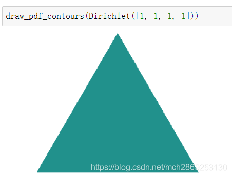
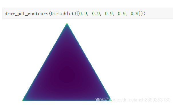
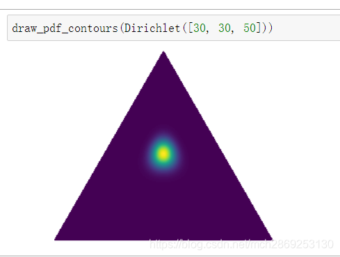
本文介绍如何使用Python的matplotlib库来绘制等边三角形网格上的Dirichlet概率密度函数轮廓图。首先定义了三角形网格及其重心坐标系转换方法，接着通过Dirichlet类实现概率密度函数的计算，并最终绘制出轮廓图。

摘要生成于 C知道，由 DeepSeek-R1 满血版支持，前往体验 >

%matplotlib inline
import numpy as np
import matplotlib.pyplot as plt
import matplotlib.tri as tri

#生成等边三角形
corners = np.array([[0, 0], [1, 0], [0.5, 0.75**0.5]])
triangle = tri.Triangulation(corners[:, 0], corners[:, 1])

#每条边中点位置
midpoints = [(corners[(i + 1) % 3] + corners[(i + 2) % 3]) / 2.0 for i in range(3)]

def xy2bc(xy, tol=1.e-3):
    #将三角形顶点的笛卡尔坐标映射到重心坐标系
    s = [(corners[i] - midpoints[i]).dot(xy - midpoints[i]) / 0.75 for i in range(3)]
    return np.clip(s, tol, 1.0 - tol)

#有了重心坐标，可以计算Dirichlet概率密度函数的值
class Dirichlet(object):
    
    def __init__(self, alpha):
        from math import gamma
        from operator import mul
        from functools import reduce
        self._alpha = np.array(alpha)
        self._coef = gamma(np.sum(self._alpha)) / reduce(mul, [gamma(a) for a in self._alpha]) #reduce:sequence连续使用function
        
    def pdf(self, x):
        #返回概率密度函数值
        from operator import mul
        from functools import reduce
        return self._coef * reduce(mul, [xx ** (aa - 1) for (xx, aa)in zip(x, self._alpha)])
    
def draw_pdf_contours(dist, nlevels=200, subdiv=8, **kwargs):
    import math
    
    #细分等边三角形网格
    refiner = tri.UniformTriRefiner(triangle)
    trimesh = refiner.refine_triangulation(subdiv=subdiv)
    pvals = [dist.pdf(xy2bc(xy)) for xy in zip(trimesh.x, trimesh.y)]

    plt.tricontourf(trimesh, pvals, nlevels, **kwargs)
    plt.axis('equal')
    plt.xlim(0, 1)
    plt.ylim(0, 0.75**0.5)
    plt.axis('off')

在这里插入图片描述