


pytorch快速学习
tensor拼接代码
示例一:
代码
import torch
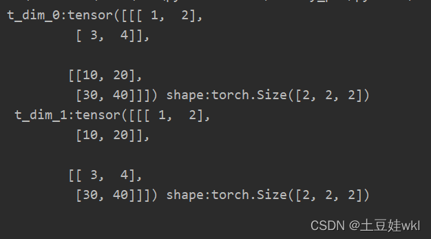
t1 = torch.tensor([(1, 2), (3, 4)])
t2 = torch.tensor([(10, 20), (30, 40)])
t_dim_0 = torch.stack([t1, t2], dim=0)
t_dim_1 = torch.stack([t1, t2], dim=1)
print("t_dim_0:{} shape:{}\n t_dim_1:{} shape:{}\n".format(t_dim_0, t_dim_0.shape, t_dim_1, t_dim_1.shape))
结果图
示例二:
代码
import torch
# 假设是时间步T1的输出
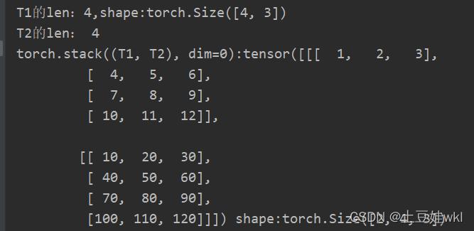
T1 = torch.tensor([[1, 2, 3],
[4, 5, 6],
[7, 8, 9], [10, 11, 12]])
print("T1的len:{},shape:{}".format(len(T1), T1.shape))
# 假设是时间步T2的输出
T2 = torch.tensor([[10, 20, 30],
[40, 50, 60],
[70, 80, 90], [100, 110, 120]])
print("T2的len:", len(T2))
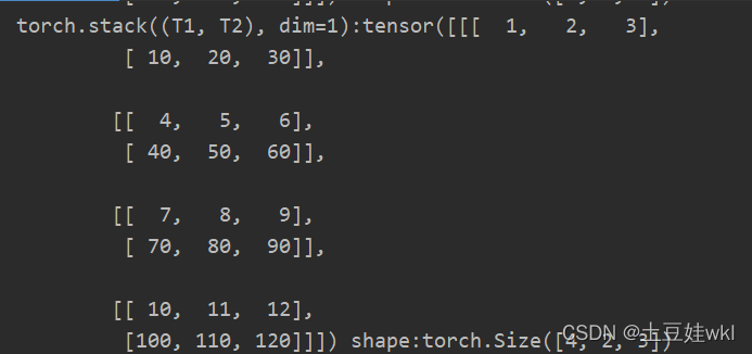
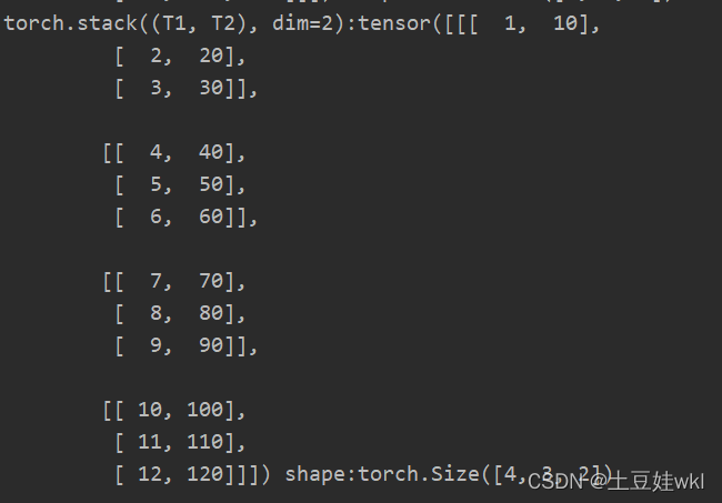
print("torch.stack((T1, T2), dim=0):{} shape:{} \ntorch.stack((T1, T2), dim=1):{} shape:{}\ntorch.stack((T1, T2), "
"dim=2):{} shape:{}\n".format(
torch.stack((T1, T2), dim=0), torch.stack((T1, T2), dim=0).shape, torch.stack((T1, T2), dim=1),
torch.stack((T1, T2), dim=1).shape, torch.stack((T1, T2), dim=2), torch.stack((T1, T2), dim=2).shape))
结果
示例三:
import torch
torch.manual_seed(1)
# flag = True
flag = False
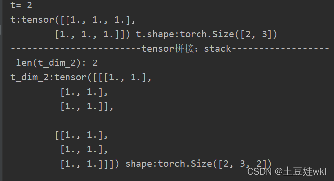
t = torch.ones(2, 3)
print("t=",len(t))
print("t:{} t.shape:{}".format(t, t.shape))
if flag:
print("------------------tensor的拼接:cat-----------------")
t_0 = torch.cat([t, t], dim=0)
t_1 = torch.cat([t, t], dim=1)
print("t_0:{} shape= {}\nt_1:{} shape= {}\n".format(t_0, t_0.shape, t_1, t_1.shape))
print("------------------------tensor拼接:stack------------------")
flag = True
# flag = False
if flag:
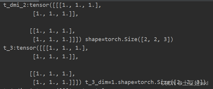
t_2 = torch.stack([t, t], dim=0)
t_3 = torch.stack([t, t], dim=1)
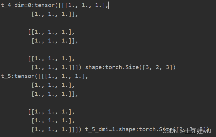
t_4 = torch.stack([t, t, t], dim=0)
t_5 = torch.stack([t, t, t], dim=1)
t_dim_2 = torch.stack([t, t], dim=2)
print(" t_dim_2:", len(t_dim_2))
print("t_dim_2:{} shape:{}\n".format(t_dim_2, t_dim_2.shape))
print("t_2:{} shape={}\nt_3:{} t_3.shape={}\nt_4_dim=0:{} shape:{}\nt_5:{} t_5.shape:{}".format(t_2, t_2.shape, t_3,
t_3.shape, t_4,
t_4.shape, t_5,
t_5.shape))
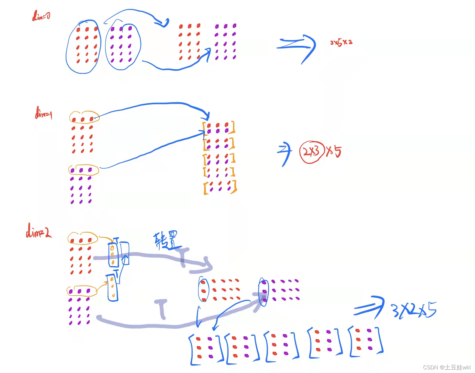
结果图:
t ensor stack拼接理解图
1、 采用torch.from_numpy创建张量,并打印查看ndarray和张量数据的地址
import numpy as np
import torch
# 创建ndarray数组
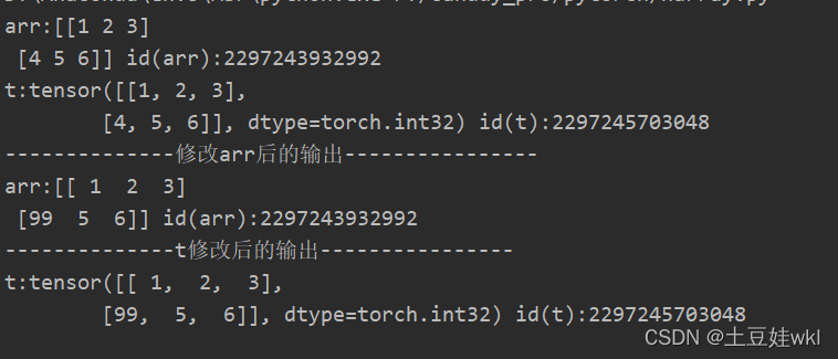
arr = np.array([[1, 2, 3], [4, 5, 6]])
print("arr:{} id(arr):{}".format(arr, id(arr)))
# ndarray 转tensor
t = torch.from_numpy(arr)
print("t:{} id(t):{}".format(t, id(t)))
arr[1, 0] = 99
print("--------------修改arr后的输出----------------")
print("arr:{} id(arr):{}".format(arr, id(arr)))
print("--------------t修改后的输出----------------")
print("t:{} id(t):{}".format(t, id(t)))
结果图:
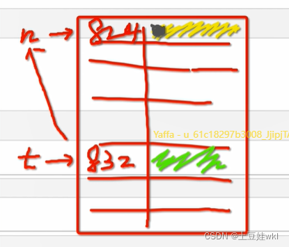
利用from_numpy与tensor共享数据内存 分析图
注意知识点
答:torch.from.numpy(ndarray)
功能:从numpy创建tensor
注意事项:从torch.from_numpy创建的tensor与原ndarray共享内存,当修改其中一个数据时,另外一个也将被改动
2、torch.normal()创建张量的四种模式
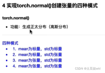
标量、 张量、向量
标量是只有大小没有方向的量简单来说就是数字1,2,3,4,5,在Python中,常用的标量类型包含字符串、数值、bool
向量就是有大小有方向的值例如(1,2)
矩阵就是好几个向量简单来说就是[[1,2,3],[4,5,6],[7,8,9],[10,11,12]]
张量就是任何量,标量,向量,矩阵就是0、1、2阶的张量
import torch
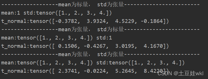
print("------------------mean为标量, std为张量------------------------")
mean = 1
std = torch.arange(1, 5, dtype=torch.float)
t_normal = torch.normal(mean, std)
print("mean:{} std:{} \nt_normal:{}".format(mean, std, t_normal))
print("------------------mean为张量, std为标量------------------------")
mean = torch.arange(1, 5, dtype=torch.float)
std = 1
t_normal = torch.normal(mean, std)
print("mean:{} std:{} \nt_normal:{}".format(mean, std, t_normal))
print("------------------mean为张量, std为张量------------------------")
mean = torch.arange(1, 5, dtype=torch.float)
std = torch.arange(1, 5, dtype=torch.float)
t_normal = torch.normal(mean, std)
print("mean:{} std:{} \nt_normal:{}".format(mean, std, t_normal))
结果:
采用broadcast机制:
当mean为标量,std为张量时候:eg:mean=1,而std=torch.arange(1, 5,dtype=torch.float)时候,mean自动会变成1x4的张量(1.,1., 1., 1.),与std:tensor([1., 2., 3., 4.])对应正态分布
作业:

1线性回归模型
调整线性回归模型停止条件以及y =2*x+(5+ torch.randn(2o,1)中的斜率,训练一个线性回归模型
1、答案:
知识点一:torch.manual_seed()
torch.manual_seed(args.seed) #为CPU设置种子用于生成随机数,以使得结果是确定的
if args.cuda:
torch.cuda.manual_seed(args.seed)#为当前GPU设置随机种子;
如果使用多个GPU,应该使用torch.cuda.manual_seed_all()为所有的GPU设置种子。
原文链接:https://blog.youkuaiyun.com/xiasli123/article/details/102645689
知识点二:float(“inf”)
Python中可以用如下方式表示正负无穷:
float(“inf”), float("-inf")
知识点三:torch.rand和torch.randn有什么区别?
一个均匀分布,一个是标准正态分布。
代码:
import torch
import matplotlib.pyplot as plt
torch.manual_seed(10)
# 线性回模型
lr = 0.01
best_loss = float("inf")
# 创建训练数据
x = torch.rand(200, 1) * 10
y = 3 * x + (5 + torch.randn(200, 1))
# 构建线性回归参数
w = torch.randn((1), requires_grad=True)
b = torch.zeros((1), requires_grad=True)
for iteration in range(10000):
# 前向传播
wx = torch.mul(w, x)
y_pred = torch.add(wx, b)
# 计算MSE loss
loss = (0.5 * (y - y_pred) ** 2).mean()
# 反向传播
loss.backward()
current_loss = loss.item()
if current_loss < best_loss:
best_loss = current_loss
best_w = w
best_b = b
# 绘图
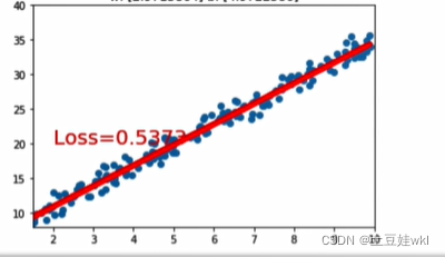
if loss.data.numpy() < 3:
plt.scatter(x.data.numpy(), y.data.numpy())
plt.plot(x.data.numpy(), y_pred.data.numpy(), 'r-', lw=5)
plt.text(2, 20, 'Loss=%.4f' % loss.data.numpy(), fontdict={'size': 20, 'color': 'red'})
plt.xlim(1.5, 10)
plt.ylim(8, 40)
plt.title('lteration:{}\nw:{}b:{}'.format(iteration, w.data.numpy(), b.data.numpy()))
plt.pause(0.5)
if loss.data.numpy() < 0.55:
break
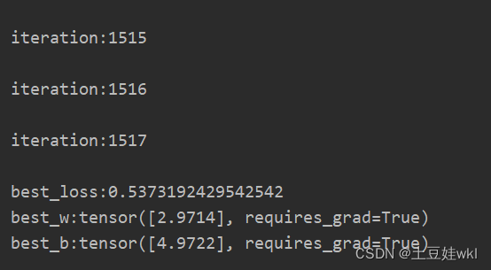
print("\niteration:{}".format(iteration))
# 更新参数
b.data.sub_(lr * b.grad)
w.data.sub_(lr * w.grad)
print("\nbest_loss:{}\nbest_w:{}\nbest_b:{}".format(best_loss, best_w, best_b))
结果图
2、答案:

3、答案


自动求导、逻辑回归homework
1、逻辑回归模型为什么可以进行二分类?
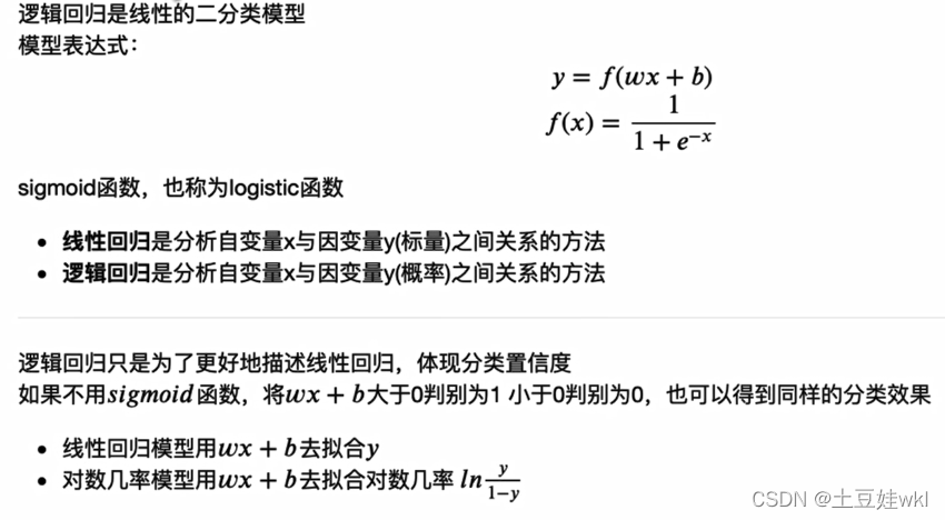
2、逻辑回归模型代码实现
采用代码实现逻辑回归模型的训练,并尝试调整数据生成中的mean_value,将mean_value设置为更小的值,例如1,或者更大的值,例如5,会出现什么情况?再尝试仅调整bias,将bias调为更大或者负数,模型训练过程是怎么样的?
2.1、代码部分—改变均值和方差去理解一下模型
import torch
import torch.nn as nn
import matplotlib.pyplot as plt
import numpy as np
torch.manual_seed(10)

# ======------------------step 1/5生成数据======
sample_nums = 100
mean_value = 1
bias = 1
n_data = torch.ones(sample_nums, 2)
x_0 = torch.normal(mean_value * n_data, 1) + bias
y_0 = torch.zeros(sample_nums)
x_1 = torch.normal(-mean_value*n_data, 1) + bias
y_1 = torch.ones(sample_nums)
train_x = torch.cat((x_0, x_1), 0)
train_y = torch.cat([y_0, y_1], 0)
max_x = torch.max(train_x)

#========step 2/5选择模型----------------
class LR(nn.Module):
    def __init__(self):
        super(LR, self).__init__()
        self.features = nn.Linear(2, 1)
        self.sigmoid = nn.Sigmoid()

    def forward(self, x):
        x = self.features(x)
        x = self.sigmoid(x)
        return x


lr_net = LR() #实例化逻辑回归模型
# --------------step 3/5选择损失函数------
loss_fn = nn.BCELoss()

#-------------step 4/5选择优化器-------
lr = 0.01
optimizer = torch.optim.SGD(lr_net.parameters(), lr=lr, momentum=0.9)


# ------------step 5/5模型训练-----
for iteration in range(1000):
    #前向传播
    y_pred = lr_net(train_x)

    # 计算loss
    loss = loss_fn(y_pred.squeeze(), train_y)

     # 反向传播
    loss.backward()

    # 更新参数
    optimizer.step()

    # 清空梯度
    optimizer.zero_grad()

    #绘图
    if iteration % 20 ==0:
        mask = y_pred.ge(0.5).float().squeeze() # 以0.5为阈值进行分类
        correct = (mask == train_y).sum() #计算正确预测的样本个数
        acc = correct.item() /train_y.size(0) #计算分类准确率

        plt.scatter(x_0.data.numpy()[:, 0], x_0.data.numpy()[:, 1], c='r', label='class 0')
        plt.scatter(x_1.data.numpy()[:, 0], x_1.data.numpy()[:, 1], c='b', label='class 1')

        w_0, w_1 = lr_net.features.weight[0]
        w_0, w_1 = float(w_0.item()), float(w_1.item())
        plot_b = float(lr_net.features.bias[0].item())
        plot_x = np.arange(torch.min(x_1[:, 1]), torch.max(x_0[:, 0]), 0.1)
        plot_y = (-w_0 * plot_x - plot_b) / w_1

        plt.xlim(torch.min(x_1[:,0]), torch.max(x_0[:, 0]))
        plt.ylim(torch.min(x_1[:, 1]), torch.max(x_0[:, 1]))
        plt.plot(plot_x, plot_y)

        plt.text(torch.min(x_1[:,0])-5, torch.max(x_0[:, 1])-5, 'Loss=%.4f' % loss.data.numpy(), fontdict={'size': 20, 'color':'red'})
        plt.title("Iteration:{}\nw_0:{:.2f} w_1:{:.2f} b:{:.2f} accuracy:{:.2%}".format(iteration, w_0, w_1, plot_b, acc))
        plt.legend()

        plt.show()
        plt.pause(0.5)

        if acc > 0.99:
            break


 1688
1688

 被折叠的 条评论
为什么被折叠?
被折叠的 条评论
为什么被折叠?
 到【灌水乐园】发言


