import os
import random
import numpy as np
import matplotlib.pyplot as plt
from PIL import Image
import torch
import torch.nn as nn
import torch.optim as optim
from torch.utils.data import Dataset, DataLoader
from torchvision import transforms
import torch.nn.functional as F
from torchsummary import summary
from sklearn.metrics import classification_report, confusion_matrix, precision_recall_fscore_support
import seaborn as sns # 新增:用于绘制混淆矩阵热力图
# 设置随机种子确保结果可复现
def set_seed(seed=42):
random.seed(seed)
np.random.seed(seed)
torch.manual_seed(seed)
torch.cuda.manual_seed(seed)
torch.backends.cudnn.deterministic = True
torch.backends.cudnn.benchmark = False
set_seed()
# 数据加载模块,修改__getitem__返回图像路径
class DigitDataset(Dataset):
def __init__(self, root_dir, transform=None, is_test=False):
self.root_dir = root_dir
self.transform = transform
self.is_test = is_test
self.classes = sorted(os.listdir(root_dir))
self.samples = []
# 构建样本列表
for class_idx, class_name in enumerate(self.classes):
class_dir = os.path.join(root_dir, class_name)
if not os.path.isdir(class_dir):
continue
for img_name in os.listdir(class_dir):
if img_name.endswith('.png'):
img_path = os.path.join(class_dir, img_name)
self.samples.append((img_path, class_idx))
# 处理类别不平衡
if not is_test:
self._balance_classes()
def _balance_classes(self):
# 统计各类样本数量
class_counts = [0] * len(self.classes)
for _, class_idx in self.samples:
class_counts[class_idx] += 1
# 找出最大样本数
max_count = max(class_counts)
# 复制少数类样本
balanced_samples = []
for class_idx in range(len(self.classes)):
class_samples = [s for s in self.samples if s[1] == class_idx]
# 复制样本直到达到最大数量
while len(class_samples) < max_count:
class_samples.extend(
random.sample(class_samples, min(len(class_samples), max_count - len(class_samples))))
balanced_samples.extend(class_samples[:max_count])
# 打乱样本顺序
random.shuffle(balanced_samples)
self.samples = balanced_samples
def __len__(self):
return len(self.samples)
def __getitem__(self, idx):
img_path, label = self.samples[idx]
image = Image.open(img_path).convert('L') # 转为灰度图
if self.transform:
image = self.transform(image)
return image, label, img_path # 新增:返回图像路径用于错误样本可视化
# 数据预处理
train_transform = transforms.Compose([
transforms.RandomRotation(10), # 随机旋转
transforms.RandomAffine(degrees=0, translate=(0.1, 0.1)), # 随机平移
transforms.ToTensor(), # 转为张量并归一化到[0,1]
transforms.Normalize((0.5,), (0.5,)) # 标准化
])
test_transform = transforms.Compose([
transforms.ToTensor(),
transforms.Normalize((0.5,), (0.5,))
])
# 加载数据集
enhanced_dir = "增强后样本"
original_dir = "测试样本"
# 创建数据集
full_dataset = DigitDataset(enhanced_dir, transform=train_transform)
# 划分训练集和验证集
train_size = int(0.8 * len(full_dataset))
val_size = len(full_dataset) - train_size
train_dataset, val_dataset = torch.utils.data.random_split(full_dataset, [train_size, val_size])
# 创建测试集,修改数据加载器以获取图像路径
test_dataset = DigitDataset(original_dir, transform=test_transform, is_test=True)
# 创建数据加载器
batch_size = 64
train_loader = DataLoader(train_dataset, batch_size=batch_size, shuffle=True, num_workers=4)
val_loader = DataLoader(val_dataset, batch_size=batch_size, shuffle=False, num_workers=4)
test_loader = DataLoader(test_dataset, batch_size=batch_size, shuffle=False, num_workers=4)
# 定义ResNet轻量化版本模型
class BasicBlock(nn.Module):
expansion = 1
def __init__(self, in_channels, out_channels, stride=1):
super(BasicBlock, self).__init__()
self.conv1 = nn.Conv2d(in_channels, out_channels, kernel_size=3, stride=stride, padding=1, bias=False)
self.bn1 = nn.BatchNorm2d(out_channels)
self.relu = nn.ReLU(inplace=True)
self.conv2 = nn.Conv2d(out_channels, out_channels, kernel_size=3, stride=1, padding=1, bias=False)
self.bn2 = nn.BatchNorm2d(out_channels)
self.shortcut = nn.Sequential()
if stride != 1 or in_channels != self.expansion * out_channels:
self.shortcut = nn.Sequential(
nn.Conv2d(in_channels, self.expansion * out_channels, kernel_size=1, stride=stride, bias=False),
nn.BatchNorm2d(self.expansion * out_channels)
)
def forward(self, x):
out = self.relu(self.bn1(self.conv1(x)))
out = self.bn2(self.conv2(out))
out += self.shortcut(x)
out = self.relu(out)
return out
class LightResNet(nn.Module):
def __init__(self, block=BasicBlock, num_blocks=[2, 2], num_classes=10):
super(LightResNet, self).__init__()
self.in_channels = 16
self.conv1 = nn.Conv2d(1, 16, kernel_size=3, stride=1, padding=1, bias=False)
self.bn1 = nn.BatchNorm2d(16)
self.relu = nn.ReLU(inplace=True)
self.layer1 = self._make_layer(block, 16, num_blocks[0], stride=1)
self.layer2 = self._make_layer(block, 32, num_blocks[1], stride=2)
self.avg_pool = nn.AdaptiveAvgPool2d((7, 7))
self.fc1 = nn.Linear(32 * block.expansion * 7 * 7, 128)
self.dropout = nn.Dropout(0.5)
self.fc2 = nn.Linear(128, num_classes)
def _make_layer(self, block, out_channels, num_blocks, stride):
strides = [stride] + [1] * (num_blocks - 1)
layers = []
for stride in strides:
layers.append(block(self.in_channels, out_channels, stride))
self.in_channels = out_channels * block.expansion
return nn.Sequential(*layers)
def forward(self, x):
out = self.relu(self.bn1(self.conv1(x)))
out = self.layer1(out)
out = self.layer2(out)
out = self.avg_pool(out)
out = out.view(out.size(0), -1)
out = self.dropout(self.fc1(out))
out = self.fc2(out)
return out
# 绘制网络拓扑图
def visualize_network(model):
# 设置中文字体支持
plt.rcParams["font.family"] = "SimHei" # 使用 SimHei 显示中文
plt.rcParams["axes.unicode_minus"] = False # 正常显示负号
plt.figure(figsize=(15, 10))
# 网络层信息
layers = [
{"name": "输入", "type": "input", "shape": (1, 28, 28)},
{"name": "卷积层1", "type": "conv", "kernel": 3, "stride": 1, "padding": 1, "filters": 16,
"shape": (16, 28, 28)},
{"name": "BatchNorm", "type": "bn", "shape": (16, 28, 28)},
{"name": "ReLU", "type": "relu", "shape": (16, 28, 28)},
{"name": "残差块1", "type": "residual", "sub_blocks": 2, "shape": (16, 28, 28)},
{"name": "残差块2", "type": "residual", "sub_blocks": 2, "shape": (32, 14, 14)},
{"name": "全局平均池化", "type": "pool", "shape": (32, 7, 7)},
{"name": "展平", "type": "flatten", "shape": (1568,)},
{"name": "全连接层1", "type": "fc", "neurons": 128, "dropout": 0.5},
{"name": "全连接层2", "type": "fc", "neurons": 10, "activation": "softmax"}
]
# 绘制网络拓扑
y_pos = np.linspace(0, 1, len(layers))
colors = {
"input": "lightblue",
"conv": "lightgreen",
"bn": "lightyellow",
"relu": "lightpink",
"residual": "mediumpurple",
"pool": "lightgray",
"flatten": "lightsalmon",
"fc": "lightskyblue"
}
for i, layer in enumerate(layers):
x_start = 0.1
width = 0.8
# 绘制层矩形
plt.fill_between([x_start, x_start + width], y_pos[i] - 0.05, y_pos[i] + 0.05,
color=colors.get(layer["type"], "white"), alpha=0.7, edgecolor='black')
# 添加层名称
plt.text(x_start + width / 2, y_pos[i], layer["name"], ha='center', va='center', fontweight='bold')
# 添加层信息
info = ""
if layer["type"] == "input":
info = f"输入形状: {layer['shape']}"
elif layer["type"] == "conv":
info = f"卷积核: {layer['kernel']}x{layer['kernel']}, 步长: {layer['stride']}, 填充: {layer['padding']}, 输出通道: {layer['filters']}"
elif layer["type"] == "residual":
info = f"{layer['sub_blocks']}个子块, 输出形状: {layer['shape']}"
elif layer["type"] == "fc":
info = f"神经元: {layer['neurons']}"
if "dropout" in layer:
info += f", Dropout: {layer['dropout']}"
if "activation" in layer:
info += f", 激活函数: {layer['activation']}"
else:
if "shape" in layer:
info = f"输出形状: {layer['shape']}"
plt.text(x_start + width / 2, y_pos[i] - 0.03, info, ha='center', va='center', fontsize=9)
# 绘制连接线(除了第一个层)
if i > 0:
plt.plot([x_start, x_start], [y_pos[i - 1] + 0.05, y_pos[i] - 0.05], 'k-', alpha=0.5)
plt.axis('off')
plt.title('网络拓扑图')
plt.tight_layout()
plt.savefig('network_topology.png')
plt.show()
# 可视化训练过程
def visualize_training(train_losses, train_accs, val_losses, val_accs):
# 设置中文字体支持
plt.rcParams["font.family"] = "SimHei" # 使用 SimHei 显示中文
plt.rcParams["axes.unicode_minus"] = False # 正常显示负号
epochs = range(1, len(train_losses) + 1)
# 创建一个2x1的子图
fig, (ax1, ax2) = plt.subplots(2, 1, figsize=(10, 12))
# 绘制损失曲线
ax1.plot(epochs, train_losses, 'b-', label='训练损失')
ax1.plot(epochs, val_losses, 'r-', label='验证损失')
ax1.set_title('训练和验证损失')
ax1.set_xlabel('轮次')
ax1.set_ylabel('损失')
ax1.legend()
ax1.grid(True)
# 绘制准确率曲线
ax2.plot(epochs, train_accs, 'b-', label='训练准确率')
ax2.plot(epochs, val_accs, 'r-', label='验证准确率')
ax2.set_title('训练和验证准确率')
ax2.set_xlabel('轮次')
ax2.set_ylabel('准确率 (%)')
ax2.legend()
ax2.grid(True)
plt.tight_layout()
plt.savefig('training_metrics.png')
plt.show()
# 可视化混淆矩阵(增强版:包含原始混淆矩阵和错误率热力图)
def visualize_enhanced_confusion_matrix(cm, class_names=None):
# 设置中文字体支持
plt.rcParams["font.family"] = "SimHei" # 使用 SimHei 显示中文
plt.rcParams["axes.unicode_minus"] = False # 正常显示负号
if class_names is None:
class_names = [str(i) for i in range(len(cm))]
# 创建两个子图:原始混淆矩阵和错误率矩阵
fig, (ax1, ax2) = plt.subplots(1, 2, figsize=(20, 8))
# 绘制原始混淆矩阵
sns.heatmap(cm, annot=True, fmt='d', cmap='Blues', ax=ax1)
ax1.set_title('混淆矩阵')
ax1.set_xlabel('预测标签')
ax1.set_ylabel('真实标签')
ax1.set_xticklabels(class_names)
ax1.set_yticklabels(class_names)
# 计算错误率矩阵 (对角线为0,非对角线为错误数/真实类别总数)
error_matrix = cm.astype('float').copy()
for i in range(len(error_matrix)):
total = np.sum(error_matrix[i, :])
if total > 0:
error_matrix[i, :] = error_matrix[i, :] / total
error_matrix[i, i] = 0 # 对角线错误率设为0
# 绘制错误率矩阵热力图
sns.heatmap(error_matrix, annot=True, fmt='.2f', cmap='Reds', ax=ax2)
ax2.set_title('类别间错误率热力图')
ax2.set_xlabel('预测标签')
ax2.set_ylabel('真实标签')
ax2.set_xticklabels(class_names)
ax2.set_yticklabels(class_names)
plt.tight_layout()
plt.savefig('confusion_matrix_enhanced.png')
plt.show()
# 可视化错误样本并分析原因
def analyze_misclassified_samples(model, data_loader, device, class_names=None, num_samples=20):
"""按类别收集误分类样本,确保每类及错误原因多样性"""
if class_names is None:
class_names = [str(i) for i in range(10)]
model.eval()
misclassified = []
error_reasons = []
class_collected = {i: 0 for i in range(10)} # 记录每类已收集的样本数
reason_types = set() # 记录已覆盖的错误原因
with torch.no_grad():
for inputs, targets, paths in data_loader:
inputs, targets = inputs.to(device), targets.to(device)
outputs = model(inputs)
_, predicted = torch.max(outputs, 1)
# 遍历当前 batch 的样本
for i in range(len(predicted)):
if predicted[i] != targets[i]:
true_label = targets[i].item()
pred_label = predicted[i].item()
# 跳过已收集足够样本的类别
if class_collected[true_label] >= 2: # 每类最多收集 2 个样本
continue
# 提取图像数据
img = inputs[i].cpu().squeeze().numpy()
path = paths[i]
# 分析错误原因
reason = _analyze_error_reason(img, true_label, pred_label)
# 优先保留新错误原因或未收集满的类别
if reason not in reason_types or class_collected[true_label] == 0:
misclassified.append({
'image': img,
'true_label': true_label,
'predicted_label': pred_label,
'path': path
})
error_reasons.append(reason)
class_collected[true_label] += 1
reason_types.add(reason)
# 满足总数则提前终止
if len(misclassified) >= num_samples:
break
if len(misclassified) >= num_samples:
break
# 兜底:若样本不足,补充剩余(避免某类无样本)
if len(misclassified) < num_samples:
for inputs, targets, paths in data_loader:
inputs, targets = inputs.to(device), targets.to(device)
outputs = model(inputs)
_, predicted = torch.max(outputs, 1)
for i in range(len(predicted)):
if predicted[i] != targets[i]:
true_label = targets[i].item()
if class_collected[true_label] >= 2:
continue
img = inputs[i].cpu().squeeze().numpy()
path = paths[i]
reason = _analyze_error_reason(img, true_label, pred_label)
misclassified.append({
'image': img,
'true_label': true_label,
'predicted_label': pred_label,
'path': path
})
error_reasons.append(reason)
class_collected[true_label] += 1
if len(misclassified) >= num_samples:
break
if len(misclassified) >= num_samples:
break
if not misclassified:
print("没有找到误分类的样本!")
return [], []
# 可视化逻辑(保持原逻辑,仅调整排版适配多类别)
plt.figure(figsize=(16, len(misclassified) * 1.5))
for i, sample in enumerate(misclassified):
plt.subplot(len(misclassified), 3, i * 3 + 1)
plt.imshow(sample['image'], cmap='gray')
plt.title(f"真实: {class_names[sample['true_label']]}\n预测: {class_names[sample['predicted_label']]}")
plt.axis('off')
plt.figtext(0.1, 0.95 - i * 0.12, f"路径: {os.path.basename(sample['path'])}", fontsize=8)
plt.figtext(0.4, 0.95 - i * 0.12, f"错误原因: {error_reasons[i]}", fontsize=8)
# 预测概率分布可视化(复用原逻辑)
if hasattr(model, 'fc2'):
img_tensor = torch.tensor(sample['image'], dtype=torch.float32).unsqueeze(0).unsqueeze(0).to(device)
img_tensor = transforms.Normalize((0.5,), (0.5,))(img_tensor)
x = model.conv1(img_tensor)
x = model.bn1(x)
x = model.relu(x)
x = model.layer1(x)
x = model.layer2(x)
x = model.avg_pool(x)
x = x.view(x.size(0), -1)
features = model.fc1(x)
logits = model.fc2(model.dropout(features))
probs = F.softmax(logits.detach(), dim=1).cpu().numpy()[0]
plt.subplot(len(misclassified), 3, i * 3 + 2)
x_axis = np.arange(len(class_names))
plt.bar(x_axis, probs, color='skyblue')
plt.xticks(x_axis, class_names, rotation=45, fontsize=6)
plt.title('预测概率分布')
plt.ylim(0, 1)
plt.figtext(0.7, 0.95 - i * 0.12,
f"真实标签概率: {probs[sample['true_label']]:.2f}\n"
f"预测标签概率: {probs[sample['predicted_label']]:.2f}",
fontsize=8)
plt.tight_layout(rect=[0, 0, 1, 0.95])
plt.suptitle('误分类样本分析(按类别&原因覆盖)', fontsize=14, fontweight='bold')
plt.savefig('misclassified_samples_analysis.png')
plt.show()
# 错误原因统计
print("\n错误原因统计:")
from collections import Counter
reason_counter = Counter(error_reasons)
for reason, count in reason_counter.most_common():
print(f"- {reason}: {count}个样本 ({count / len(error_reasons) * 100:.1f}%)")
return misclassified, error_reasons
def _analyze_error_reason(img, true_label, pred_label):
"""启发式分析错误原因"""
# 1. 检查图像是否有噪声(基于像素值分布)
noise_threshold = 0.15 # 噪声比例阈值
pixel_values = img.flatten()
non_zero_pixels = pixel_values[pixel_values > 0.1] # 忽略接近黑色的像素
if len(non_zero_pixels) > 0:
std = np.std(non_zero_pixels)
mean = np.mean(non_zero_pixels)
noise_ratio = std / mean if mean > 0 else 0
else:
noise_ratio = 0
# 2. 检查图像是否有极端变形(基于边界框分析)
# 找到数字的边界框
rows, cols = np.where(img > 0.1)
if len(rows) == 0 or len(cols) == 0:
return "图像为空或几乎全黑"
height = max(rows) - min(rows) + 1
width = max(cols) - min(cols) + 1
aspect_ratio = height / width if width > 0 else float('inf')
normal_aspect = 1.0 # 正常数字的宽高比
deformation_threshold = 1.5 # 变形阈值
# 3. 检查是否为相似数字对(如3和8,1和7等)
similar_pairs = [(3, 8), (8, 3), (1, 7), (7, 1), (2, 7), (7, 2), (4, 9), (9, 4)]
# 4. 检查笔画是否模糊(基于梯度幅度)
# 计算水平和垂直梯度
dx = np.gradient(img, axis=1)
dy = np.gradient(img, axis=0)
gradient_magnitude = np.sqrt(dx ** 2 + dy ** 2)
edge_pixels = gradient_magnitude[gradient_magnitude > 0.1]
edge_clarity = np.mean(edge_pixels) if len(edge_pixels) > 0 else 0
# 综合判断错误原因
if (true_label, pred_label) in similar_pairs:
return f"相似数字混淆({true_label}与{pred_label})"
elif noise_ratio > noise_threshold:
return "噪声干扰导致识别错误"
elif abs(aspect_ratio - normal_aspect) > deformation_threshold:
return "极端变形(宽高比异常)"
elif edge_clarity < 0.2:
return "笔画模糊导致识别困难"
elif height < 10 or width < 10:
return "数字过小或残缺"
else:
return "其他原因(可能是手写风格极端)"
# 训练函数
def train(model, train_loader, criterion, optimizer, epoch, device):
model.train()
running_loss = 0.0
correct = 0
total = 0
for batch_idx, (inputs, targets, _) in enumerate(train_loader):
inputs, targets = inputs.to(device), targets.to(device)
optimizer.zero_grad()
outputs = model(inputs)
loss = criterion(outputs, targets)
loss.backward()
optimizer.step()
running_loss += loss.item()
_, predicted = outputs.max(1)
total += targets.size(0)
correct += predicted.eq(targets).sum().item()
if (batch_idx + 1) % 50 == 0:
print(f'Epoch: {epoch + 1}, Batch: {batch_idx + 1}/{len(train_loader)}, '
f'Loss: {running_loss / (batch_idx + 1):.4f}, '
f'Train Acc: {100. * correct / total:.2f}%')
return running_loss / len(train_loader), 100. * correct / total
# 验证函数
def validate(model, val_loader, criterion, device):
model.eval()
running_loss = 0.0
correct = 0
total = 0
with torch.no_grad():
for inputs, targets, _ in val_loader:
inputs, targets = inputs.to(device), targets.to(device)
outputs = model(inputs)
loss = criterion(outputs, targets)
running_loss += loss.item()
_, predicted = outputs.max(1)
total += targets.size(0)
correct += predicted.eq(targets).sum().item()
val_loss = running_loss / len(val_loader)
val_acc = 100. * correct / total
print(f'Val Loss: {val_loss:.4f}, Val Acc: {val_acc:.2f}%')
return val_loss, val_acc
# 测试函数(增强版:返回详细指标和误分类样本)
def enhanced_test(model, test_loader, device, class_names=None):
"""执行测试并返回详细评估指标和误分类样本"""
if class_names is None:
class_names = [str(i) for i in range(10)]
model.eval()
correct = 0
total = 0
all_targets = []
all_predicted = []
all_paths = [] # 存储图像路径用于错误分析
with torch.no_grad():
for inputs, targets, paths in test_loader:
inputs, targets = inputs.to(device), targets.to(device)
outputs = model(inputs)
_, predicted = outputs.max(1)
total += targets.size(0)
correct += predicted.eq(targets).sum().item()
all_targets.extend(targets.cpu().numpy())
all_predicted.extend(predicted.cpu().numpy())
all_paths.extend(paths)
test_acc = 100. * correct / total
print(f'Test Acc: {test_acc:.2f}%')
# 计算精确率、召回率、F1分数
precision, recall, f1, _ = precision_recall_fscore_support(
all_targets, all_predicted, average=None)
avg_precision = np.mean(precision)
avg_recall = np.mean(recall)
avg_f1 = np.mean(f1)
# 打印详细指标
print("\n详细评估指标:")
print(f"测试集准确率: {test_acc:.2f}%")
print(f"平均精确率: {avg_precision:.4f}")
print(f"平均召回率: {avg_recall:.4f}")
print(f"平均F1分数: {avg_f1:.4f}")
# 打印分类报告
print("\n分类报告:")
print(classification_report(all_targets, all_predicted, target_names=class_names))
# 计算混淆矩阵
cm = confusion_matrix(all_targets, all_predicted)
# 找出误分类样本
misclassified_indices = np.where(np.array(all_targets) != np.array(all_predicted))[0]
misclassified_samples = []
for idx in misclassified_indices[:20]: # 最多取20个样本
misclassified_samples.append({
'image_path': all_paths[idx],
'true_label': all_targets[idx],
'predicted_label': all_predicted[idx]
})
return {
'accuracy': test_acc,
'precision': precision,
'recall': recall,
'f1': f1,
'average_precision': avg_precision,
'average_recall': avg_recall,
'average_f1': avg_f1,
'confusion_matrix': cm,
'misclassified_samples': misclassified_samples
}
if __name__ == '__main__':
# 初始化模型
device = torch.device("cuda" if torch.cuda.is_available() else "cpu")
model = LightResNet().to(device)
# 打印模型结构
print("模型结构:")
summary(model, (1, 28, 28))
# 定义损失函数和优化器
criterion = nn.CrossEntropyLoss()
optimizer = optim.Adam(model.parameters(), lr=0.001, betas=(0.9, 0.999))
scheduler = optim.lr_scheduler.ReduceLROnPlateau(optimizer, 'min', patience=3, factor=0.5)
# 训练模型
epochs = 10
best_val_acc = 0.0
best_model_path = 'best_model.pth'
# 记录训练过程
train_losses, train_accs = [], []
val_losses, val_accs = [], []
for epoch in range(epochs):
print(f'\nEpoch {epoch + 1}/{epochs}')
train_loss, train_acc = train(model, train_loader, criterion, optimizer, epoch, device)
val_loss, val_acc = validate(model, val_loader, criterion, device)
# 记录训练过程
train_losses.append(train_loss)
train_accs.append(train_acc)
val_losses.append(val_loss)
val_accs.append(val_acc)
# 学习率调整
scheduler.step(val_loss)
# 保存最佳模型
if val_acc > best_val_acc:
best_val_acc = val_acc
torch.save(model.state_dict(), best_model_path)
print(f'模型已保存,验证准确率: {best_val_acc:.2f}%')
# 加载最佳模型并进行增强测试
model.load_state_dict(torch.load(best_model_path, weights_only=True))
test_results = enhanced_test(model, test_loader, device)
# 可视化增强版混淆矩阵(包含错误率热力图)
class_names = [str(i) for i in range(10)]
visualize_enhanced_confusion_matrix(test_results['confusion_matrix'], class_names)
# 可视化训练结果(保持原有功能)
visualize_training(train_losses, train_accs, val_losses, val_accs)
visualize_network(model)
# 可视化误分类样本并分析原因
print("\n分析误分类样本...")
misclassified_samples, error_reasons = analyze_misclassified_samples(
model, test_loader, device, class_names, num_samples=10)
# 输出最常见的错误类型
if misclassified_samples:
print("\n最常见的错误类型:")
from collections import Counter
reason_counter = Counter(error_reasons)
top_reasons = reason_counter.most_common(3)
for reason, count in top_reasons:
print(f"- {reason}: {count}个样本")
阅读代码


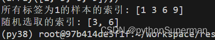
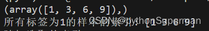
 本文介绍了Python中random.sample函数用于从序列中随机抽取不重复元素的方法,以及numpy.where用于在标签数组中选取满足条件的样本索引。同时,讲解了extend()方法在合并列表方面的应用。


 957
957

 被折叠的 条评论
为什么被折叠?
被折叠的 条评论
为什么被折叠?
 到【灌水乐园】发言


