


 本文通过实战案例介绍如何运用正则化线性回归进行数据拟合,并探讨不同正则化参数对模型偏差-方差的影响。
在这篇博文中我们将会实现正则化的线性回归以及利用他去学习模型,不同的模型会具有不同的偏差-方差性质,我们将研究正则化以及偏差和方差之间的相互关系和影响。
这一部分的数据是关于通过一个水库的水位来预测水库的流水量。为了进行偏差和方差的检验,这里用12组数据进行回归而用交叉数据集中的21组数据进行验证。
正则化的线性回归(Regularized Linear Regression)
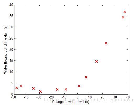
首先这12组数据由上图展现出来,下面进行线性回归。
正则化线性回归代价函数
正则化的线性回归的代价函数为
其中 λ λ 是控制正则化程度的参数。正则化项是作为代价函数中惩罚项存在的。这里需要注意的是 θ0 θ 0 并不需要正则化。
正则化线性回归梯度函数
对应地,正则化线性函数对于
θj
θ
j
的偏导定义为
拟合线性回归
在这么小的数据规模下正则化项的用处将不会很明显,这里设置为0.然后利用fmincg函数求得
J(θ)
J
(
θ
)
的最小值,得到下面的回归直线。
训练
θ
θ
的函数如下
function [theta] = trainLinearReg(X, y, lambda)
%TRAINLINEARREG Trains linear regression given a dataset (X, y) and a
%regularization parameter lambda
%   [theta] = TRAINLINEARREG (X, y, lambda) trains linear regression using
%   the dataset (X, y) and regularization parameter lambda. Returns the
%   trained parameters theta.
%

% Initialize Theta
initial_theta = zeros(size(X, 2), 1);

% Create "short hand" for the cost function to be minimized
costFunction = @(t) linearRegCostFunction(X, y, t, lambda);

% Now, costFunction is a function that takes in only one argument
options = optimset('MaxIter', 200, 'GradObj', 'on');

% Minimize using fmincg
theta = fmincg(costFunction, initial_theta, options);

end
以及调用的
function [J, grad] = linearRegCostFunction(X, y, theta, lambda)
%LINEARREGCOSTFUNCTION Compute cost and gradient for regularized linear
%regression with multiple variables
%   [J, grad] = LINEARREGCOSTFUNCTION(X, y, theta, lambda) computes the
%   cost of using theta as the parameter for linear regression to fit the
%   data points in X and y. Returns the cost in J and the gradient in grad

% Initialize some useful values
m = length(y); % number of training examples

% You need to return the following variables correctly
J = 0;
grad = zeros(size(theta));

% ====================== YOUR CODE HERE ======================
% Instructions: Compute the cost and gradient of regularized linear
%               regression for a particular choice of theta.
%
%               You should set J to the cost and grad to the gradient.
%


h = X*theta;
J = (1/(2*m))*sum((h-y).^2) + (lambda/(2*m))*sum(theta(2:end,:).^2);

grad(1,:) =(1/m)*sum((h-y) .* X(:,1));

for c = 2:size(theta,1)
  grad(c,:) = (1/m)*sum((h-y) .* X(:,c)) + (lambda/m)*(theta(c,:));

end

% =========================================================================

end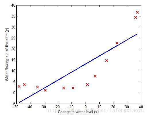
由于给定的数据并不是线性的,因此线性回归的效果是一般的,那么如何衡量回归效果的好坏呢,主要依赖于两个指标:偏差(Bias)和方差(variance)
偏差(Bias)-方差(variance)
关于偏差和方差,可以通过绘制训练误差和测试误差机型评判,通过学习曲线来判断两个指标的变化。参考如下博客
学习曲线
绘制学习曲线,我们需要针对不同的训练(training)集规模有训练(training error)和交叉验证集合误差(cross validation set error)。为了获得不同的训练集规模,需要利用原始训练集
X
X
的不同子集。特别地,我们可以用前个例子(例如
X(1:i,:)
X
(
1
:
i
,
:
)
和
y(1:i)
y
(
1
:
i
)
)
首先训练
θ
θ
,之后计算两个误差,其中训练误差由下式定义
特别地,训练误差不包括正则化项。当利用 λ λ 计算训练误差和交叉验证误差时,将其设置为0。当计算训练集误差的时候,选择的是一个子集。然而对于交叉验证集误差,选择的是全集。
学习曲线的MATLAB程序为
function [error_train, error_val] = ...
    learningCurve(X, y, Xval, yval, lambda)
%LEARNINGCURVE Generates the train and cross validation set errors needed
%to plot a learning curve
%   [error_train, error_val] = ...
%       LEARNINGCURVE(X, y, Xval, yval, lambda) returns the train and
%       cross validation set errors for a learning curve. In particular,
%       it returns two vectors of the same length - error_train and
%       error_val. Then, error_train(i) contains the training error for
%       i examples (and similarly for error_val(i)).
%
%   In this function, you will compute the train and test errors for
%   dataset sizes from 1 up to m. In practice, when working with larger
%   datasets, you might want to do this in larger intervals.
%

% Number of training examples
m = size(X, 1);

% You need to return these values correctly
error_train = zeros(m, 1);
error_val   = zeros(m, 1);

% ====================== YOUR CODE HERE ======================
% Instructions: Fill in this function to return training errors in
%               error_train and the cross validation errors in error_val.
%               i.e., error_train(i) and
%               error_val(i) should give you the errors
%               obtained after training on i examples.
%
% Note: You should evaluate the training error on the first i training
%       examples (i.e., X(1:i, :) and y(1:i)).
%
%       For the cross-validation error, you should instead evaluate on
%       the _entire_ cross validation set (Xval and yval).
%
% Note: If you are using your cost function (linearRegCostFunction)
%       to compute the training and cross validation error, you should
%       call the function with the lambda argument set to 0.
%       Do note that you will still need to use lambda when running
%       the training to obtain the theta parameters.
%
% Hint: You can loop over the examples with the following:
%
%       for i = 1:m
%           % Compute train/cross validation errors using training examples
%           % X(1:i, :) and y(1:i), storing the result in
%           % error_train(i) and error_val(i)
%           ....
%
%       end
%

% ---------------------- Sample Solution ----------------------

for i = 1:m
X_sub = X(1:i, :);
 y_sub = y(1:i);

 theta = trainLinearReg(X_sub, y_sub, lambda);

error_train(i) = linearRegCostFunction(X_sub, y_sub, theta, 0);
error_val(i) = linearRegCostFunction(Xval, yval, theta, 0);
end


% -------------------------------------------------------------

% =========================================================================

end
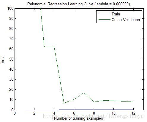
下面对正则化线性回归绘制学习曲线
%% =========== Part 5: Learning Curve for Linear Regression =============
%  Next, you should implement the learningCurve function.
%
%  Write Up Note: Since the model is underfitting the data, we expect to
%                 see a graph with "high bias" -- slide 8 in ML-advice.pdf
%

lambda = 0;
[error_train, error_val] = ...
    learningCurve([ones(m, 1) X], y, ...
                  [ones(size(Xval, 1), 1) Xval], yval, ...
                  lambda);

plot(1:m, error_train, 1:m, error_val);
title('Learning curve for linear regression')
legend('Train', 'Cross Validation')
xlabel('Number of training examples')
ylabel('Error')
axis([0 13 0 150])

fprintf('# Training Examples\tTrain Error\tCross Validation Error\n');
for i = 1:m
    fprintf('  \t%d\t\t%f\t%f\n', i, error_train(i), error_val(i));
end

%fprintf('Program paused. Press enter to continue.\n');
%pause;
得到
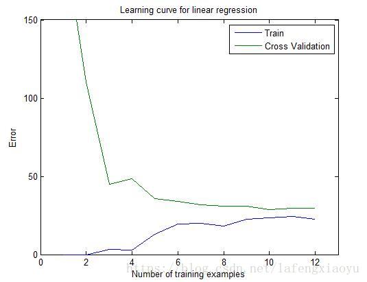
可以从上图看出两个误差在训练数目增加的时候都很高。这是因为只用线性回归拟合的模型过于简单,很难拟合地很好。
多项式回归
与之前二分类的问题类似,我们对自变量做
p
p
次回归,便可以得到如下的多项式回归形式。
需要用原有的数据相乘 1—p 1 — p 次形成 p p 次特征
学习多项式回归
进行多项式回归,对于上面处理好的次数据,由于乘方的原因会导致和之前的数据相比有很大的数量级上的差别。因此还需要一步特征标准化,用下面的函数进行标准化,记录相应的 μ μ 和 σ σ
function [X_norm, mu, sigma] = featureNormalize(X)
%FEATURENORMALIZE Normalizes the features in X
%   FEATURENORMALIZE(X) returns a normalized version of X where
%   the mean value of each feature is 0 and the standard deviation
%   is 1. This is often a good preprocessing step to do when
%   working with learning algorithms.

mu = mean(X);
X_norm = bsxfun(@minus, X, mu);

sigma = std(X_norm);
X_norm = bsxfun(@rdivide, X_norm, sigma);
% ============================================================

end
虽然在特征向量中我们利用的是多项式项,但是事实上还是在解决线性回归问题。依然可以利用上面的方法求解相应的
θ
θ
值。
结合学习到的
θ
θ
值,绘制回归曲线如下图
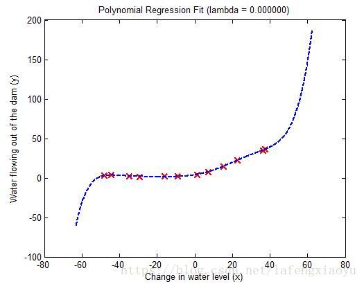
可以看出拟合的效果是不错的,但是1.拟合曲线非常复杂2.在两边的数据往外都会有断崖式的上升和下降。这都说明曲线存在过拟合现象。
从学习曲线也可以看出。训练集合误差是非常小的,但是交叉验证误差却很大。说明训练误差和交叉验证误差之间存在很大差距,也就意味着高方差(variance)。其中一种解决过拟合的方式就是增加正则化项
调整正则化参数
分别设置正则化参数 λ λ 为1和100的回归曲线和学习曲线分别为
| λ=1 λ = 1 回归曲线 | λ=1 λ = 1 学习曲线 |
|---|---|
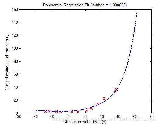 | 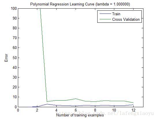 |
在
λ=1
λ
=
1
时,数据拟合的效果是不错的。而且从学习曲线也可以看出并没有出现很高的偏差和方差,说明
λ=1
λ
=
1
取得了很好的偏差-方差平衡(trade-off)。
| λ=100 λ = 100 回归曲线 | λ=100 λ = 100 学习曲线 |
|---|---|
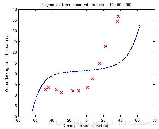 | 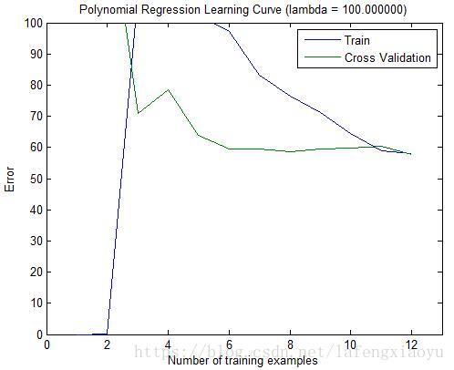 |
而
λ=100
λ
=
100
时正则化项比重过高会导致拟合效果很差。
正则化系数的选择
这里给出了
λ={0;0:001;0:003;0:01;0:03;0:1;0:3;1;3;10}
λ
=
{
0
;
0
:
001
;
0
:
003
;
0
:
01
;
0
:
03
;
0
:
1
;
0
:
3
;
1
;
3
;
10
}
,通过绘制两个误差的走势衡量哪个
λ
λ
是最优选择。
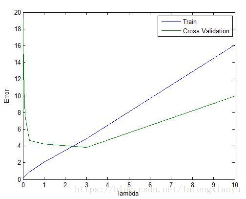
我们可以选择 λ=3 λ = 3 ,这个时候的训练集合误差和交叉验证误差都不大。
计算测试集误差
为了验证“最后”参数选择的效果,最好使利用没有参与过任何参数训练的集合进行评估。这里选择交叉验证集的数据进行交叉验证。
lambda = 3;
[theta] = trainLinearReg(X_poly, y, lambda);%之前X_poly已经添加了全1列了,无需在添加了
error3_test=linearRegCostFunction(X_poly_test,ytest,theta,0);
fprintf('the test error is %f\n',error3_test);
fprintf('Program paused. Press enter to continue.\n');
pause;
得到测试误差为 3.8599 3.8599
利用随机选择的例子绘制学习曲线
在实践中,特别是小的训练集,需要绘制学习曲线以验证算法的时候,经常会随机选择例子进行交叉验证之后取其平均值。
具体而言,对于
i
i
个例子,为了确定训练误差和交叉验证误差,需要首先从两个集合中分别随机选择个例子。然后利用训练集中的
i
i
个例子学习参数并且用交叉验证集中的个例子进行验证。重复50次,取其两个误差的平均误差为最终的两个误差。
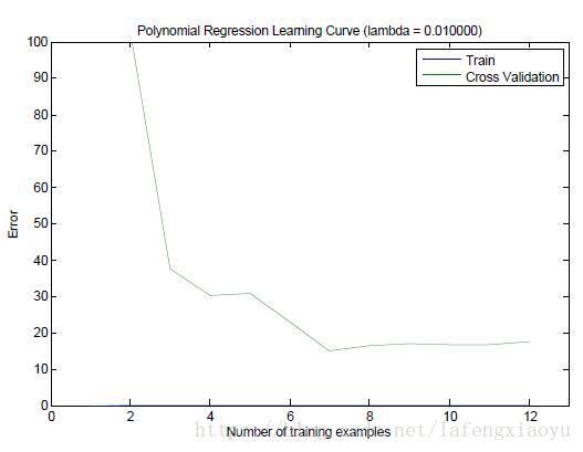
上图是取 λ=0.01 λ = 0.01 进行随机选择的学习曲线,由于随机选择的集合每次都可能是不一样的,因此可能绘制出略微有些区别的曲线~~


 679
679

 被折叠的 条评论
为什么被折叠?
被折叠的 条评论
为什么被折叠?
 到【灌水乐园】发言


