Attention Is All You Need论文解读

2 Background

The goal of reducing sequential computation also forms the foundation of the Extended Neural GPU
[16], ByteNet [18] and ConvS2S [9], all of which use convolutional neural networks as basic building
block, computing hidden representations in parallel for all input and output positions. In these models,
the number of operations required to relate signals from two arbitrary input or output positions grows
in the distance between positions, linearly for ConvS2S and logarithmically for ByteNet. This makes
it more difficult to learn dependencies between distant positions [12]. 在Transformer中这个过程被减少为常数级别的操作， albeit at the cost of reduced effective resolution due to averaging attention-weighted positions, an effect we counteract with Multi-Head Attention as described in section 3.2.

Self-attention, 有时也称为intra-attention，是一种将单个序列中不同位置关联起来的attention机制，最终目的是计算得到关于这个序列的一种表示方式。Self-attention已经在许多任务中得到了成功应用，包括reading comprehension, abstractive summarization, textual entailment 以及 learning task-independent sentence representations [4, 27, 28, 22].

End-to-end memory networks are based on a recurrent attention mechanism instead of sequencealigned recurrence and have been shown to perform well on simple-language question answering and
language modeling tasks [34].

据我们所知，Transformer是第一个完全依赖self-attention机制，不使用sequencealigned RNNs or convolution来计算输入输出representation的transduction model。

3 Model Architecture

Most competitive neural sequence transduction models有一个encoder-decoder结构[5, 2, 35]。 这里，encoder将输入序列的符号表示$(x_1,\dots ,x_n)$映射为连续的序列化表达$z=(z_1,\dots ,z_n)$。给定$z$后，decoder接下来按每步一个的顺序生成输出符号序列$y_1,\dots ,y_m)$。在每一步模型都是auto-regressive [10]的，consuming the previously generated symbols as additional input when generating the next.

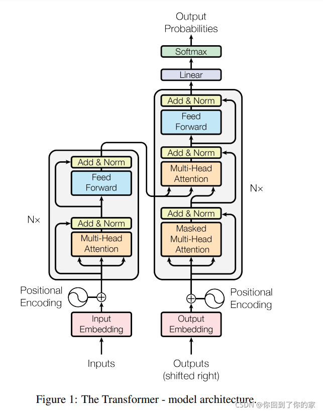
Transformer同样遵循上述结构，对encoder和decoder都使用堆叠的self-attention and point-wise, fully connected layers。如图1左右所示：

3.1 Encoder and Decoder Stacks

Encoder

上图中左侧为encoder块，右侧为decoder块。橙色部分为Multi-Head Attention，这由多个Self-Attention组成，我们可以看到Encoder块包含一个Multi-Head Attention，而Decoder块包含两个Multi-Head Attention（其中一个用到Masked）。Multi-Head Attention上方还包括一个Add&Norm层，Add表示残差连接用于防止网络退化，Norm表示Layer Normalization，用于对每一层的激活值进行归一化。以一个例子说明，假设我们在encoder input处的输入是机器学习，在decoder input中输入的是，输出是machine。在下一个时刻decoder input的输入是machine，输出是learning，不断重复直到输出是句点（。），代表翻译结束。

接下来看encoder和decoder内部分别做了什么，先看左半部分的encoder：我们输入$X\in R(n_x,N)$通过一个input Embedding的转移矩阵$W_x\in R(d,n_x)$变成了一个张量，这个张量就是上文的embedding $I\in R(d,N)$，接下来我们加上一个表示位置的positional encoding $E\in R(d,N)$，得到一个张量，接下来进行后面的操作。

张量进入绿色的块后会重复N次。绿色的块中第一层是multi-head attention，一个序列$I\in R(d,N)$经过multi-head attention后，我们可以得到另外一个序列$O\in R(d,N)$

接下来进行Add&Norm，这个意思是，将multi-head attention层的输入$I\in R(d,N)$和输出$O\in R(d,N)$进行相加后，再进行Layer Normalization，Layer Normalizaiton和Batch Normalizaiton的区别见如下两个图：

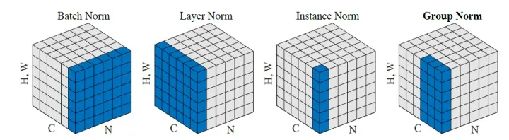
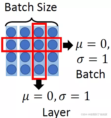
其中，Batch Normalization和Layer Normalization的对比可以概括为上图，Batch Normalization强行让一个batch的数据的某个channel的$\mu =0,\sigma =1$ ，而Layer Normalization让一个数据的所有channel的$\mu =0,\sigma =1$ 。下图也是说明了ayer Normalizaiton和Batch Normalizaiton的区别：

接下来跟着的是一个Feed Forward的前馈网络和一个Add&Norm层，所以，绿色块中前两个层的操作表示为：

$$O_1=LayerNormalization(I+MultiheadSelfAttention(I))$$

这一绿色块的后两层操作的表达式为：
$$O_2=LayerNormalization(O_1+FeedForwardNetwork(O_1))$$

整体可以表示为：

$$Block(I)=O_2$$

所以transformer的encoder整体操作为：

$$Encoder(I)=Block(...Block(Block(I)))Ntimes$$

在论文中，设定$N=6$，为了实现残差连接，模型中的所有子层（包括embedding层）的输出都是512维，即$d_{model}=512$。

Decoder

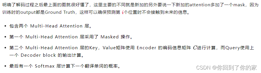
Decoder的输入包括两部分，下方是前一个time step的输出embedding，即上文所述的$I\in R(d,N)$，再加上一个表示位置的positional embedding $E\in R(d,N)$，得到一个张量，接下来进行后面的操作。即进入绿色块，首先进行Masked Multi-Head Self-Attention，masked的意思是使得attention只会attend on 已经产生的序列，这个很合理，因为还没有产生出来的东西不存在，无法进行attention。

输出是对应$i$位置的输出词的概率分布。

输入是：Encoder的输出和对应$i-1$位置的decoder的输出，所以中间的attention不是self-attention，它的key和value来自encoder，query来自上一位置decoder的输出。

这里要特别注意一下，编码可以并行计算，一次性全部encoding出来，但解码不是一次把所有序列解出来的，而是像RNN一样一个一个解出来的，因为要用上一个位置的输入当作attention的query。

下面详细介绍下Masked Multi-Head Self-attention的具体操作，Masked在Scale操作之后，softmax操作之前。

因为在翻译的过程中是顺序翻译的，即翻译完第i个单词，才可以翻译第$i+1$个单词。通过maked操作可以防止第i个单词获取到第i+1个单词的信息。下面以 “我有一只猫” 翻译成 “I have a cat” 为例，了解一下 Masked 操作。在 Decoder 的时候，是需要根据之前的翻译，求解当前最有可能的翻译，如下图所示。首先根据输入 “” 预测出第一个单词为 “I”，然后根据输入 " I" 预测下一个单词 “have”。

待补充

decoder同样由 $N=6$ 个相同的层堆叠而成。相比于encoder层中有两个子层，decoder插入了一个新的子层，这个子层对encoder层的输出执行multi-head attention。和encoder类似，decoder中同样使用了残差连接，然后应用了layer normalization。我们同样修改了decoder层中的self-attention子层来prevent positions from attending to subsequent positions. This masking, combined with fact that the output embeddings are offset by one position, ensures that the predictions for position i can depend only on the known outputs at positions less than i.

3.2 Attention

假设我们的输入是下图的$x_1-x_4$，这是一个序列：

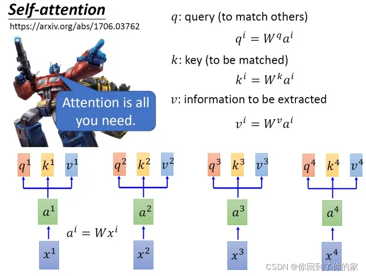
每一个输入向量先乘上一个矩阵$W$得到embedding，即向量$a_1-a_4$，接下来这个embedding进入self-attention层，每一个向量$a_1-a_4$分别乘上三个不同的转化矩阵$W_q,W_k,W_v$，以向量$a_1$为例，这时分别得到三个不同的向量$q_1,k_1,v_1$。

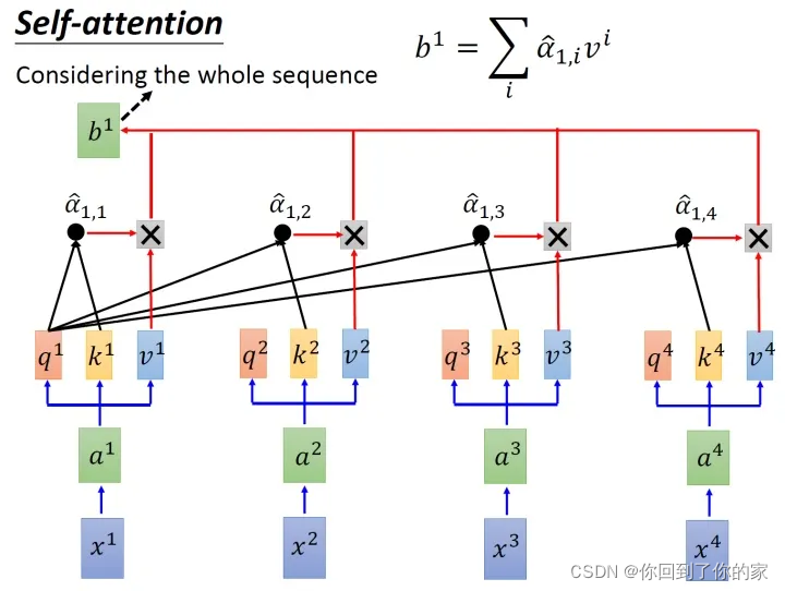
接下来我们使用每个query q去对每个key k做attention，attention本质上就是匹配这两个向量有多接近，例如我们现在对$q_1$和$k_1$做attention，我们就可以把这两个向量做scaled inner product，得到${\alpha }_{1,1}$。接下来用$a_1$和$k_2$做attention，得到${\alpha }_{1,2}$，同理得到${\alpha }_{1,3},{\alpha }_{1,4}$。上述过程可以用下图表示：

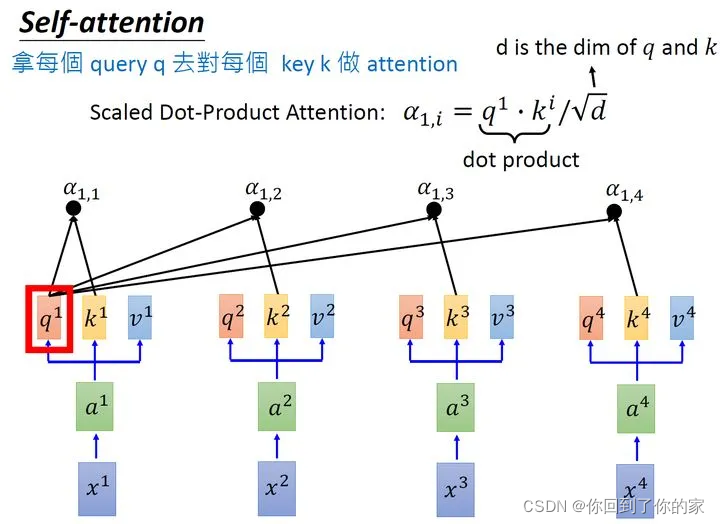
scaled inner product计算方式如下：

$${\alpha }_{1,i}=q_1\cdot k_i/\sqrt{d}$$

这里d是q和k的维度。因为$q\cdot k$的数值会随着维度的增大而增大，所以要除以$\sqrt{dimension}$的值，相当于进行了归一化。

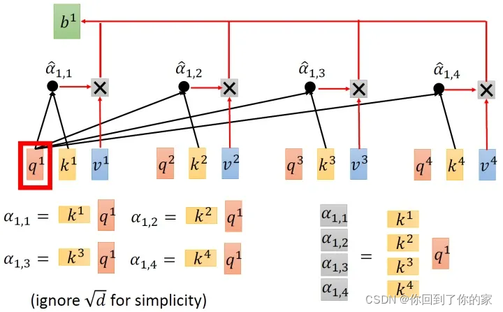
接下来的过程如图6所示，将计算得到的所有${\alpha }_{1,i}$值取softmax操作：

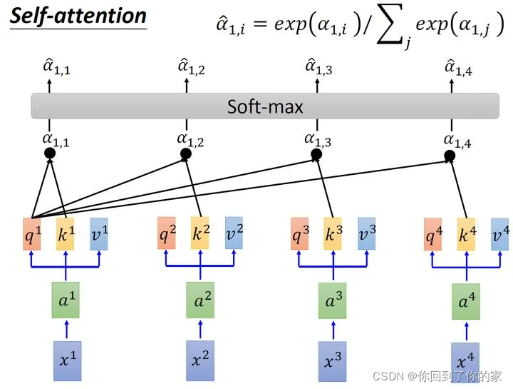
进行softmax操作后我们得到了${\hat{\alpha }}_{1,i}$，我们将它和所有$v_i$值相乘。就是用${\hat{\alpha }}_{1,1}$乘$v_1$，后面也类似，将结果进行加和得到$b_1$，所以在获取到$b_1$的过程中用到了整个序列的信息。如果仅考虑局部信息，那么仅需要学习出对应的${\hat{\alpha }}_{1,i}=0$，此时$b_1$就不再带有那个对应分支的信息了，如果需要学习全局信息，那么保证${\hat{\alpha }}_{1,i}\ne 0$，此时$b_1$就带有全部的对应分支的信息了，计算得到$b_1$的过程如下图所示：

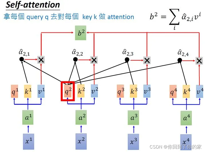
使用类似的方法，我们可以计算出$b_2$，如下图所示：

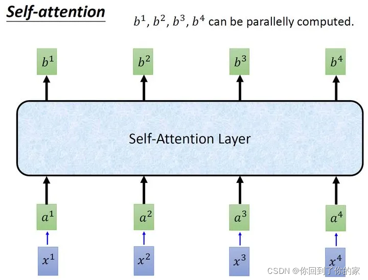
同理我们可以计算得到$b_3,b_4$。经过上述一连串计算，self-attention layer层所做的事和RNN其实是一样的，只是它可以并行计算获取结果，如下图所示：

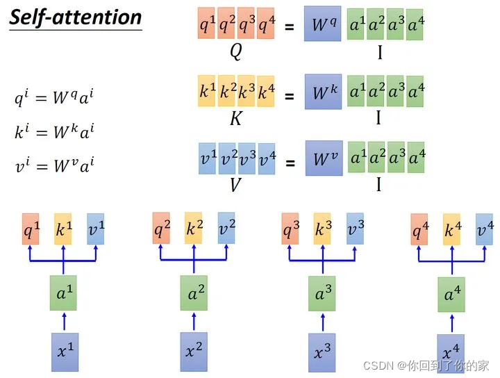
接下来我们使用矩阵表示上述过程，输入的embedding是$I=[a_1,a_2,a_3,a_4]$，我们接下来使用$I$乘以转化矩阵$W_q$得到$Q=[q_1,q_2,q_3,q_4]$，每一列都代表一个向量q。同理我们用$I$乘以转化矩阵$W_k$得到$K=[k_1,K_2,K_3,K_4]$，它的每一列都代表一个向量k。同理通过转化矩阵$W_v$我们可以得到$V=[v_1,v_2,v_3,v_4]$，它的每一列代表一个向量v。如下图所示：

接下来是k和q的attention过程，我们可以将向量k横过来变成行向量，然后列向量q做内积（省略$\sqrt{d}$）。这样$\alpha$就成了$4\times 4$的矩阵，它由4个行向量拼成的矩阵和四个列向量拼成的矩阵做内积得到，如下图所示：

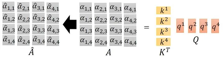
这里整个过程可以被表示为如下图所示的过程：

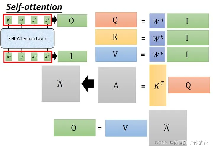
输入矩阵$I\in R(d,N)$分别乘上三个不同的矩阵$W_q,W_k,W_v\in R(d,d)$得到三个中间矩阵$Q,K,V\in R(d,N)$。它们的维度相同，将K转置之后与Q相乘得到Attention矩阵$A\in R(N,N)$，代表每一个位置两两之间的attention。再将它取softmax操作得到$\hat{A}\in R(N,N)$，最后将它乘以V矩阵得到输出向量$O\in R(d,N)$

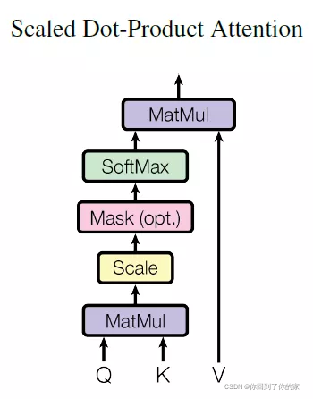
3.2.1 Scaled Dot-Product Attention

我们将我们的特定attention机制称为 “Scaled Dot-Product Attention”，如图2所示：

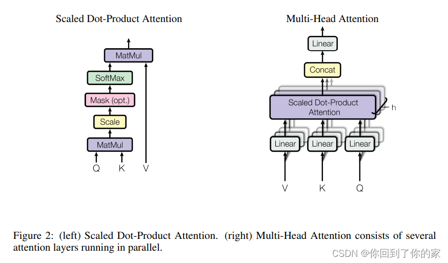
输入包括维度为$d_k$的queries、key以及维度为$d_v$的values。我们计算the dot products of the query with all keys, divide each by $\sqrt{d_k}$, and apply a softmax function to obtain the weights on the values.

实际上，我们对一组queries同时计算attention function，然后打包进一个矩阵$Q$。keys以及values同样打包进了矩阵$K$以及$V$。我们通过如下方式计算输出矩阵：

$$\text{Attention}(Q,K,V)=\text{softmax}(\frac{Q{K}^T}{\sqrt{d_k}})V(1)$$

两个最常使用的attention functions是additive attention [2]以及dot-product (multiplicative) attention. Dot-product attention 和我们的算法相同，除了缩放因子 $\frac{1}{\sqrt{d_k}}$。Additive attention通过使用一个单隐藏层前馈网络来计算compatibility function。尽管这两种attention的理论计算复杂度类似，但是dot-product attention在实际计算中明显更快并且更高效, 这是因为它可以通过高度优化的矩阵乘法代码进行实现。

尽管对于较小的$d_k$来说两种mechanism表现相似，additive attention在$d_k$较大且没有scaling时效果好于dot product attention 。我们设想对于较大的$d_k$，dot product会在量级上迅速增长，pushing the softmax function into regions where it has extremely small gradients（这里看下脚注）。为了消除这种影响，我们将dot product 缩小了尺度因子$\frac{1}{\sqrt{d_k}}$。

3.2.2 Multi-Head Attention

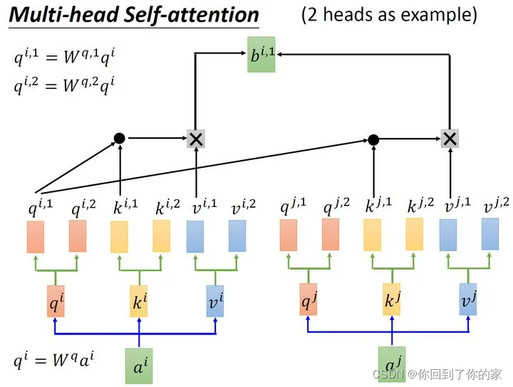
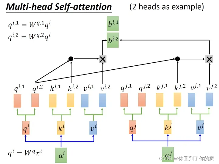
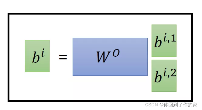
以两个head的情况为例：由$a_i$生成的$q_i$进一步乘以两个转移矩阵变为$q_{i,1}$和$q_{i,2}$，同理我们可以得到$k_{i,1}$和$k_{i,2}$，$v_{i,1}$和$v_{i,2}$。接下来$q_{i,1}$再与$k_{i,1}$进行attention，得到weighted sum的权重$\alpha$，再与$v_{i,1}$做weighted sum得到最终的$b_{i,1}(i=1,2,...,N)$。同理我们可以得到$b_{i,2}(i=1,2,...,N)$。现在我们已经获取了$b_{i,1}(i=1,2,...,N)\in R(d,1)$和$b_{i,2}(i=1,2,...,N)\in R(d,1)$，我们可以把它们拼接起来，然后通过一个转换矩阵来调整维度，使其与刚才的$b_i(i=1,2,...,N)\in R(d,1)$维度相同，整个过程如下所示：

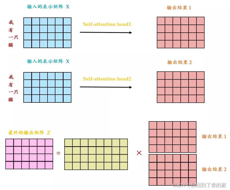
从下图中我们可以看出Multi-Head Attention包含多个Self-Attention层，首先我们将输入$X$分别传递到两个不同的Self-Attention中，计算得到两个输出矩阵，然后将这两个矩阵拼接起来传入一个线性层中，得到Multi-Head Attention的最终输出$Z$。Multi-Head Attention输出的矩阵$Z$与其输入的矩阵$X$的维度是一样的：

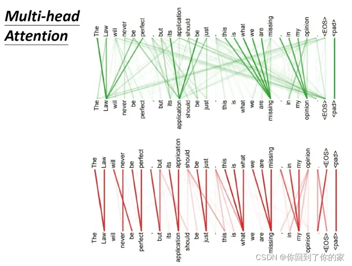
下图展示了一组Multi-Head Attention的结果，其中绿色部分是一组query和key，红色部分是另外一组query和key，我们可以发现绿色部分其实更关注global信息，而红色部分更关注local信息：

我们没有仅仅使用$d_{\text{model}}$维的keys、values以及queries的attention function，而是使用学习到的不同线性映射将queries、keys以及values分别映射 $h$ 次到 $d_k,d_k$ 以及 $d_v$ 维。对于每个映射后的queries、keys以及values我们并行计算attention function，这会生成 $d_v$ 维的输出值。然后我们将这些值拼接起来再进行映射，生成最终值，如图2所示。

Multi-head attention允许模型共同关注来自不同位置的不同representation subspaces的信息。当使用单个attention head时，averaging inhibits this。

$$\text{MultiHead}(Q,K,V)=\text{Concat}({\text{head}}_1,...,{\text{head}}_h)W^O$$
$$\text{where}{\text{head}}_i=\text{Attention}(Q{W}_i^Q,K{W}_i^K,V{W}_i^V)$$

这里映射都为参数矩阵，$W_i^Q\in {\mathbb{R}}^{d_{model}\times d_k},W_i^K\in {\mathbb{R}}^{d_{model}\times d_k},W_i^V\in {\mathbb{R}}^{d_{model}\times d_v},W^O\in {\mathbb{R}}^{h{d}_v\times d_{model}}$

在本文中，我们采用$h=8$个并行的attention layer或者head。对于每个head，我们使用$d_k=d_v=d_{model}/h=64$。由于每个head的维度都减小了，总计算花销和有全部维度的single-head attention相似。

3.2.3 模型中Attention机制的应用

Transformer中通过三种不同的方式使用了multi-head attention机制：

• 在“encoder-decoder attention”层，queries来自于之前的decoder层，memory keys和values来自于encoder的输出层。这允许decoder中的每个位置都参与输入序列中的所有位置。这模仿了sequence-to-sequence模型中经典的encoder-decoder attention机制。
• encoder包含self-attention层。在一个self-attention层中所有的keys、values以及queries都来自同一个地方，在我们的例子中，这就是encoder之前层的输出。encoder中的每个位置可以参与到encoder先前层的所有位置。
• 类似地，decoder中的self-attention层允许decoder中的每个位置参与到decoder前以及当前层的全部位置。我们需要防止decoder中的leftward information flow来组织auto-regressive。We implement this inside of scaled dot-product attention by masking out (setting to $-\infty$) all values in the input of the softmax which correspond to illegal connections. 如图2所示。

3.3 Position-wise Feed-Forward Networks

除了attention子层之外，编码器和解码器中的每一层都包含一个全连接前馈网络，该网络分别相同地应用于每个位置。这包括两个线性变换，中间有一个ReLU激活。

$$\text{FFN}(x)=\max (0,x{W}_1+b_1)W_2+b_2$$

这里线性变化的结构在不同的位置是相同的，但是每层使用不同的参数。另外一种描述这个的方式是核大小为1的两个卷积层。输入核输出的维度都是$d_{model}=512$，内层的维度为$d_{ff}=2048$。

3.4 Embedding 以及 Softmax

与其他序列转换模型类似，我们使用学习到的embeddings将输入tokens和输出tokens转换为维度为$d_{model}$的向量。我们还使用学习到的线性变换和softmax函数将decoder输出转换为预测的下一个token概率。在我们的模型中，我们在两个embedding层和pre-softmax线性变换之间共享相同的权重矩阵，类似于[30]。在embedding层中，我们将这些权重乘以$\sqrt{d_{model}}$。

3.5 Positional Encoding

self-attention有一个问题，那就是不包含位置信息，一个距离较近的单词和距离较远的单词向量效果完全一样。作者为了解决这个问题所作的操作如下图所示：


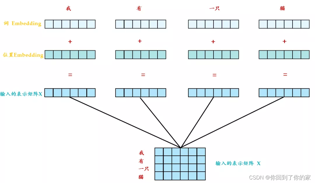
具体的做法是：给每一个位置规定一个表示位置信息的向量$e_i$，让它与$a_i$加在一起之后作为新的$a_i$参与后面的运算过程，但是注意这个$e_i$是人工设定的，不是神经网络学习出来的，因此每一个位置都有一个不同的$e_i$。

到这里有一个问题，为什么是$e_i$与$a_i$相加，而不是拼接？加起来之后，原来表示位置的信息就混杂到$a_i$里面去了，现在不是很难被找到了吗？

这里提供一种解答这个问题的思路：

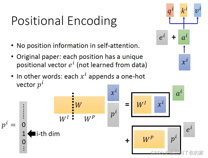
如上图所示，我们先给每个位置的$x_i\in R(d,1)$append一个one-hot编码的向量$p_i\in R(N,1)$，得到一个新的输入向量$x_p^i\in R(d+N,1)$，这个向量作为新的输入，乘上一个转化矩阵$W=[W_I,W_P]\in R(d,d+N)$，那么：

$$W\cdot x_p^i=[W_I,W_P]\cdot \left[\begin{array}{c}{x}_i\\ p_i\end{array}\right]=W_I\cdot x_i+W_P\cdot p_i=a_i+e_i$$

所以$e_i$与$a_i$相加就等于把原来的输入$x_i$concat一个表示位置的one-hot编码$p_i$，再进行转化。

这个与位置编码相乘的矩阵$W_P$是人工设计的，如下图所示：

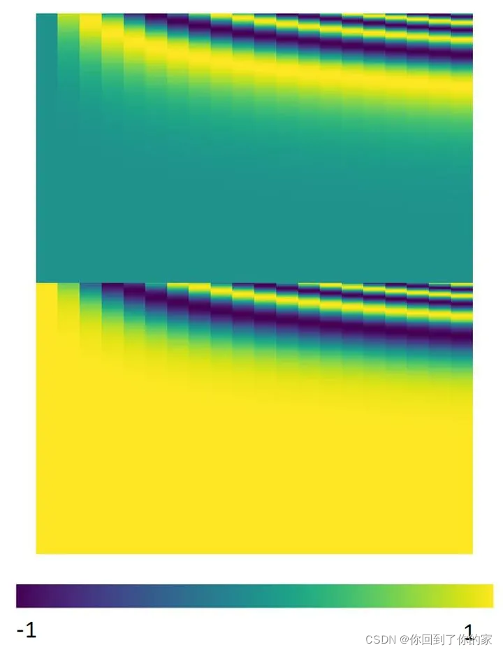
positional encodings用PE表示，它的维度与单词Embeddings相同，PE可以通过训练得到，也可以采用某种公式直接计算得到，在transformer中采用了不同频率的sine以及cosine方程，计算方式如下：

$$PE(pos,2i)=sin(pos/10000^{2i/d_{model}})$$
$$PE(pos,2i+1)=cos(pos/10000^{2i/d_{model}})$$

式中，$pos$表示token在序列中的位置，例如第一个token“我”的pos=0

i，或者准确意义上是$2i$和$2i+1$表示了PE的维度，i的取值范围是$[0,..,d_{model}/2)$。所以当pos为1时，对应的PE可以写成：

$$PE(1)=[sin(1/10000^{0/512}),cos(1/10000^{0/512}),sin(1/10000^{2/512}),cos(1/10000^{2/512}),...]$$

式中，$d_{model}=512$，底数是10000，为什么要使用10000呢，这个就类似于玄学了，原论文中完全没有提啊，这里不得不说说论文的readability的问题，即便是很多高引的文章，最基本的内容都讨论不清楚，所以才出现像上面提问里的讨论，说实话这些论文还远远没有做到easy to follow。这里我给出一个假想：$10000^{1/512}$是一个比较接近1的数（1.018），如果用100000，则是1.023。这里只是猜想一下，其实大家应该完全可以使用另一个底数。

使用上面的式子的好处是：

• 每个位置有一个唯一的PE
• 使得PE能够适应逼训练集里面所有句子更长的句子，假设训练集里面最长的句子有20个单词，突然来了一个长度为21的句子，则使用公式计算的方法可以计算出第21位的embedding。
• 可以让模型容易地计算出相对位置，对于固定长度的间距k，任意位置的$P{E}_{pos+k}$都可以被$P{E}_{pos}$的线性函数表示，因为三角函数特性：
  $$cos(\alpha +\beta )=cos(\alpha )cos(\beta )-sin(\alpha )sin(\beta )$$
  $$sin(\alpha +\beta )=sin(\alpha )cos(\beta )+cos(\alpha )sin(\beta )$$

我们同样测试了使用学习到的positional embeddings[9]，发现这两种方案会产生基本相同的结果（见表3 行E）。

4 为什么使用Self-Attention

In this section we compare various aspects of self-attention layers to the recurrent and convolutional layers commonly used for mapping one variable-length sequence of symbol representations
(x1, …, xn) to another sequence of equal length (z1, …, zn), with xi
, zi ∈ R
d
, such as a hidden
layer in a typical sequence transduction encoder or decoder. Motivating our use of self-attention we
consider three desiderata.

One is the total computational complexity per layer. Another is the amount of computation that can
be parallelized, as measured by the minimum number of sequential operations required.

The third is the path length between long-range dependencies in the network. Learning long-range
dependencies is a key challenge in many sequence transduction tasks. One key factor affecting the
ability to learn such dependencies is the length of the paths forward and backward signals have to
traverse in the network. The shorter these paths between any combination of positions in the input
and output sequences, the easier it is to learn long-range dependencies [12]. Hence we also compare
the maximum path length between any two input and output positions in networks composed of the
different layer types.

如表1所示，一个self-attention层在常数级的sequentially executed操作下连接了所有的位置，相比而言recurrent层需要$O(n)$的sequential operations。从计算复杂度的角度看来，当序列长度n小于representation dimensionality d时，self-attention层要比recurrent层快，这是绝大多数情况下会发生的（with sentence representations used by state-of-the-art models in machine translations, such as word-piece [38] and byte-pair [31] representations. ）为了提升一些包括非常长序列任务的计算性能，self-attention可以被限定为仅考虑以输出位置为中心的输入序列的某个邻域r。This would increase the maximum path length to O(n/r). We plan to investigate this approach further in future work。

A single convolutional layer with kernel width k < n does not connect all pairs of input and output
positions. Doing so requires a stack of O(n/k) convolutional layers in the case of contiguous kernels,
or O(logk(n)) in the case of dilated convolutions [18], increasing the length of the longest paths
between any two positions in the network. Convolutional layers are generally more expensive than
recurrent layers, by a factor of k. Separable convolutions [6], however, decrease the complexity
considerably, to O(k · n · d + n · d
2
). Even with k = n, however, the complexity of a separable
convolution is equal to the combination of a self-attention layer and a point-wise feed-forward layer,
the approach we take in our model.

As side benefit, self-attention could yield more interpretable models. We inspect attention distributions
from our models and present and discuss examples in the appendix. Not only do individual attention
heads clearly learn to perform different tasks, many appear to exhibit behavior related to the syntactic
and semantic structure of the sentences.