R语言决策树：NBA球员如何拿到大合同

作者：胡言  R语言中文社区专栏作者

知乎ID：https://www.zhihu.com/people/hu-yan-81-25

前言

本次实践学习并练习使用R语言rpart包构建决策树，寻找决定高薪合同的技术统计元素。

期间用到了过采样方法解决目标样本量太少的问题，并应用了AUC、KS、混肴矩阵、精确度等模型评价指标，算是决策树的一次比较完备的实例实践。

废话少说，上代码：

载入包

#载入分析所需要的包
library(dplyr)
library(devtools)
library(woe)   
library(ROSE)
library(rpart)
library(rpart.plot)
library(ggplot2)
require(caret)
library(pROC)

使用Rmarkdown写code时我喜欢把整个工程用到的包都在最开始的地方载入，可以设置(include=FALSE)不展示这部分代码，好处是通篇比较干净整洁。

本文用到的数据依旧是为2016-2017赛季NBA300多为球员的技术统计，感谢简书用户“牧羊的男孩”（点击阅读原文获取）。

以下为“牧羊的男孩”提供的数据字段解释，非常感谢！

dat_nba<-read.csv('nba_2017_nba_players_with_salary.csv')
dat_nba$cut_salary<-ifelse(dat_nba$SALARY_MILLIONS>15,1,0)
dat_nba$cut_salary<-as.factor(dat_nba$cut_salary)
dat_nba<-select(dat_nba,-PLAYER,-SALARY_MILLIONS,-TEAM)
cat('目标变量：\n')
summary(dat_nba$cut_salary)
cat('\n')
names(dat_nba)

目标变量：

1. 0 1

2. 291 51

• [1] "X" "Rk" "POSITION" "AGE" "MP" "FG"

• [7] "FGA" "FG." "X3P" "X3PA" "X3P." "X2P"

• [13] "X2PA" "X2P." "eFG." "FT" "FTA" "FT."

• [19] "ORB" "DRB" "TRB" "AST" "STL" "BLK"

• [25] "TOV" "PF" "POINTS" "GP" "MPG" "ORPM"

• [31] "DRPM" "RPM" "WINS_RPM" "PIE" "PACE" "W"

计算IV值

#install_github("riv","tomasgreif")
#library(devtools)
#library(woe)          
IV<-iv.mult(dat_nba,"cut_salary",TRUE)   #原理是以Y作为被解释变量，其他作为解释变量，建立决策树模型
iv.plot.summary(IV)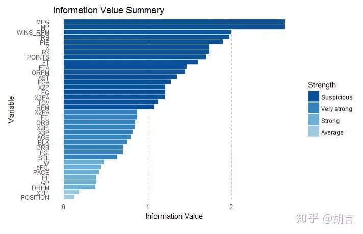

过采样办法

#install.packages("ROSE")
#library(ROSE)
# 过采样&下采样
datt1<-dat_nba
table(datt1$cut_salary)
data_balanced_both <- ovun.sample(cut_salary ~ ., data = datt1, method = "both", p=0.5,N=342,seed = 1)$data
table(data_balanced_both$cut_salary)

原始样本正负比例：

• 0 1

• 291 51

过采样后正负比例：

• 0 1

• 183 159

#library(rpart)

#设置随机分配，查分数据为train集和test集#
dat=data_balanced_both
smp_size <- floor(0.6 * nrow(dat))
set.seed(123)
train_ind <- sample(seq_len(nrow(dat)), size = smp_size)
train <- dat[train_ind, ]
test <- dat[-train_ind, ]
dim(train)
dim(test)

fit<-(cut_salary~.)
rtree<-rpart(fit,minsplit=10, cp=0.03,data=train)
printcp(rtree)

#library(rpart.plot) #调出rpart.plot包
rpart.plot(rtree, type=2)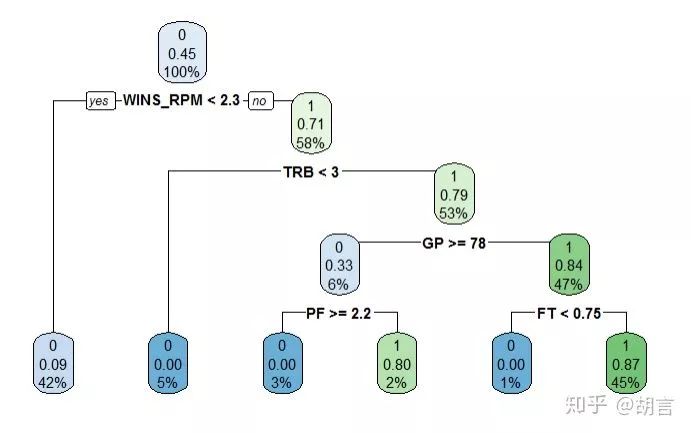 

Warning message:

In strsplit(code, "\n", fixed = TRUE) :

input string 1 is invalid in this locale

• [1] 205 37

• [1] 137 37

Classification tree:

rpart(formula = fit, data = train, minsplit = 10, cp = 0.03)

Variables actually used in tree construction:

[1] FT GP PF TRB WINS_RPM

Root node error: 93/205 = 0.45366

n= 205

CP nsplit rel error xerror xstd

• 1 0.548387 0 1.00000 1.00000 0.076646

• 2 0.118280 1 0.45161 0.50538 0.064717

• 3 0.043011 2 0.33333 0.40860 0.059826

• 4 0.032258 3 0.29032 0.34409 0.055878

• 5 0.030000 5 0.22581 0.33333 0.055156

#检验预测效果#
pre_train<-predict(rtree,type = 'vector') #type = c("vector", "prob", "class", "matrix"),
table(pre_train,train$cut_salary)

#检验test集预测效果#
pre_test<-predict(rtree, newdata = test,type = 'vector')
table(pre_test, test$cut_salary)

#检验整体集预测效果#
pre_dat<-predict(rtree, newdata = datt1,type = 'class')
table(pre_dat, datt1$cut_salary)

train集： 0 1

• 99 8

• 13 85

test集 0 1

• 60 13

• 11 53

pre_dat 0 1

• 237 10

• 54 41

评价决策树

result=datt1
result$true_label=result$MobDr1to6_od15
result$pre_prob=pre_dat
#install.packages("gmodels")
TPR <- NULL
FPR <- NULL
for(i in seq(from=1,to=0,by=-0.1)){
  #判为正类实际也为正类
  TP <- sum((result$pre_prob >= i) * (result$true_label == 1)) 
  #判为正类实际为负类
  FP <- sum((result$pre_prob >= i) * (result$true_label == 0))
  #判为负类实际为负类
  TN <- sum((result$pre_prob < i) * (result$true_label == 0)) 
  #判为负类实际为正类
  FN <- sum((result$pre_prob < i) * (result$true_label == 1)) 
  TPR <- c(TPR,TP/(TP+FN))
  FPR <- c(FPR,FP/(FP+TN))
}

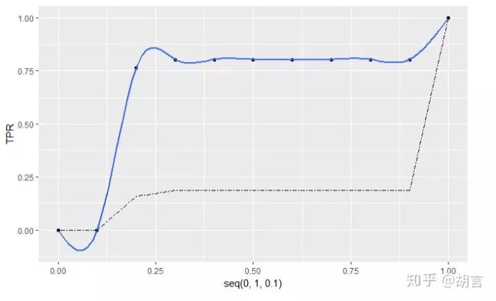
max(TPR-FPR)  #KS

#library(ggplot2)
ggplot(data=NULL,mapping = aes(x=seq(0,1,0.1),y=TPR))+
  geom_point()+
  geom_smooth(se=FALSE,formula = y ~ splines::ns(x,10), method ='lm')+
  geom_line(mapping = aes(x=seq(0,1,0.1),y=FPR),linetype=6)

KS值为：

[1] 0.3277339

# 找到KS值对应的切分点：
for (i in seq(0,10,1)){
  print(i)
  print(TPR[i]-FPR[i])
}
## 混肴矩阵
result$pre_to1<-ifelse(result$pre_prob>=0.7,1,0)
#require(caret)
xtab<-table(result$pre_to1,result$true_label)
confusionMatrix(xtab)

[1] 0

numeric(0)

• [1] 1

• [1] 0

• [1] 2

• [1] 0

• [1] 3

• [1] 0.6066303

• [1] 4

• [1] 0.6183546

• [1] 5

• [1] 0.6183546

• [1] 6

• [1] 0.6183546

• [1] 7

• [1] 0.6183546

• [1] 8

• [1] 0.6183546

• [1] 9

• [1] 0.6183546

• [1] 10

• [1] 0.6183546

Confusion Matrix and Statistics

0 1

0 237 10

1 54 41

Accuracy : 0.8129

95% CI : (0.7674, 0.8528)

No Information Rate : 0.8509

P-Value [Acc > NIR] : 0.9772

Kappa : 0.4561

Mcnemar's Test P-Value : 7.658e-08

• Sensitivity : 0.8144

• Specificity : 0.8039

• Pos Pred Value : 0.9595

• Neg Pred Value : 0.4316

• Prevalence : 0.8509

• Detection Rate : 0.6930

• Detection Prevalence : 0.7222

• Balanced Accuracy : 0.8092

• 'Positive' Class : 0

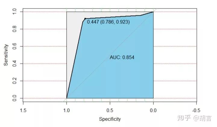
## roc曲线及AUC
#library(pROC)
datt1_pro<-predict(rtree, newdata = datt1,type = 'prob')
datt1$pre_prob<-datt1_pro[,2]
modelroc <- roc(datt1$cut_salary,datt1$pre_prob)
plot(modelroc, print.auc=TRUE, auc.polygon=TRUE, grid=c(0.1, 0.2),
     grid.col=c("green", "red"), max.auc.polygon=TRUE,
     auc.polygon.col="skyblue", print.thres=TRUE)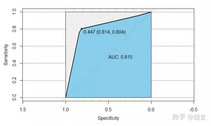

#设置随机分配，查分数据为train集和test集#
dat=datt1
smp_size <- floor(0.5 * nrow(dat))
train_ind <- sample(seq_len(nrow(dat)), size = smp_size)
train_2 <- dat[train_ind, ]
test_2 <- dat[-train_ind, ]
dim(train_2)
dim(test_2)

#检验预测效果#
pre_train_2<-predict(rtree,newdata=train_2,type = 'vector')
table(pre_train_2,train_2$cut_salary)

#检验test集预测效果#
pre_test_2<-predict(rtree, newdata = test_2,type = 'vector')

table(pre_test_2, test_2$cut_salary)

pre_train_2p<-predict(rtree,newdata=train_2,type = 'prob')
train_2$pre<-pre_train_2p[,2]
modelroc <- roc(train_2$cut_salary,train_2$pre)
plot(modelroc, print.auc=TRUE, auc.polygon=TRUE, grid=c(0.1, 0.2),
     grid.col=c("green", "red"), max.auc.polygon=TRUE,
     auc.polygon.col="skyblue", print.thres=TRUE)


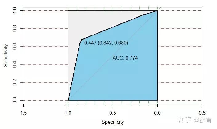
pre_test_2p<-predict(rtree, newdata = test_2,type = 'prob')
test_2$pre<-pre_test_2p[,2]
modelroc <- roc(test_2$cut_salary,test_2$pre)
plot(modelroc, print.auc=TRUE, auc.polygon=TRUE, grid=c(0.1, 0.2),
     grid.col=c("green", "red"), max.auc.polygon=TRUE,
     auc.polygon.col="skyblue", print.thres=TRUE)

• [1] 171 38

• [1] 171 38

• pre_train_2 0 1

• 1 114 2

• 2 31 24

• pre_test_2 0 1

• 1 123 8

• 2 23 17

公众号后台回复关键字即可学习

回复 爬虫             爬虫三大案例实战  
回复 Python        1小时破冰入门

回复 数据挖掘      R语言入门及数据挖掘
回复 人工智能      三个月入门人工智能
回复 数据分析师   数据分析师成长之路 
回复 机器学习      机器学习的商业应用
回复 数据科学      数据科学实战
回复 常用算法      常用数据挖掘算法