吴恩达机器学习 (线性回归)

机器学习基础详解

最新推荐文章于 2024-08-18 23:42:17 发布

原创最新推荐文章于 2024-08-18 23:42:17 发布 · 236 阅读

0 ·

CC 4.0 BY-SA版权

机器学习专栏收录该内容

5 篇文章

订阅专栏

本文深入讲解了机器学习的基本概念，包括监督学习、无监督学习、强化学习等分类，重点介绍了线性和多变量线性回归的原理及应用。通过实例演示了特征缩放、学习率调整等技巧，并对比了梯度下降法与正规方程的优缺点。

第一章: 引言

定义: 计算机程序从经验E中学习,解决任务T,进行某一性能度量P,通过P测定在T上的表现因经验E而提高.-----Tom Mitchell

分类: 监督学习, 无监督学习, 强化学习, 推荐系统

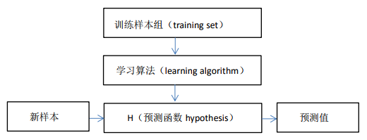
监督学习: 给算法一个数据集(有输入输出作为参考),算法从这些数据集中找出规律并帮助做出预测.

回归问题: 结果是线性的,我们设法预测出一个连续值的结果(房价问题)

分类问题: 结果是离散的,我们设法预测出一个离散值的结果(肿瘤问题)

无监督学习: 不知道输出有哪些,只能将数据进行聚类

分类聚类区别:

分类(知道有哪些类)

聚类(根据特征将数据分开)

第二章: 单变量线性回归

思路:

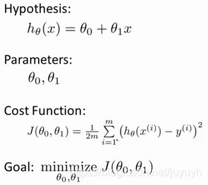
注: 2m是为了求导方便

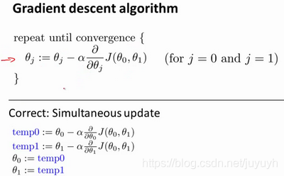
其中α是学习率（learning rate），它决定了我们沿着能让代价函数下降程度最大的方向向下迈出的步子有多大，在批量梯度下降中，我们每一次都同时让所有的参数减去学习速率乘以代价函数的导数。

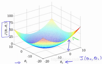
代价函数直观理解:

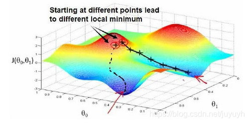
梯度下降直观理解:

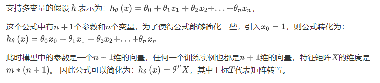
第四章: 多变量线性回归

使用矩阵,向量的思想

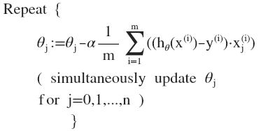
多变量梯度下降

代价函数: $J(\theta _{0},\theta _{1}...\theta _{n}) = \frac{1}{2m}\sum_{i=1}^{m}(h_{\theta }(x^{(i))})-y^{(i))})^{2}$

多变量线性回归的批量梯度下降算法为：

梯度下降法技巧

1. 特征缩放

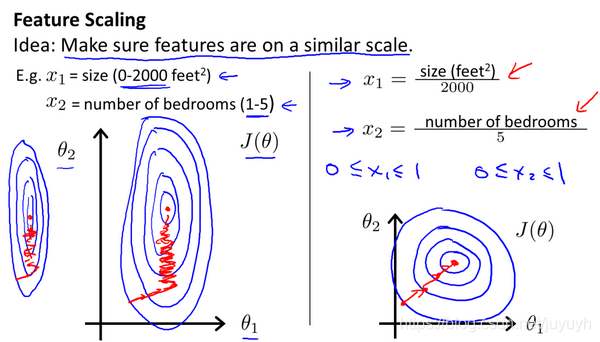
最简单的方法是令： $x_{n} = \frac{x_{n}-\mu _{n}}{s_{n}}$ ，其中 $\mu _{n}$ 是平均值， $s_{n}$ 是标准差。

2. 学习率

梯度下降算法收敛所需要的迭代次数根据模型的不同而不同，我们不能提前预知，我们可以绘制迭代次数和代价函数的图表来观测算法在何时趋于收敛。

梯度下降算法的每次迭代受到学习率的影响，如果学习率过小，则达到收敛所需的迭代次数会非常高；如果学习率过大，每次迭代可能不会减小代价函数，可能会越过局部最小值导致无法收敛。

特征和多项式回归

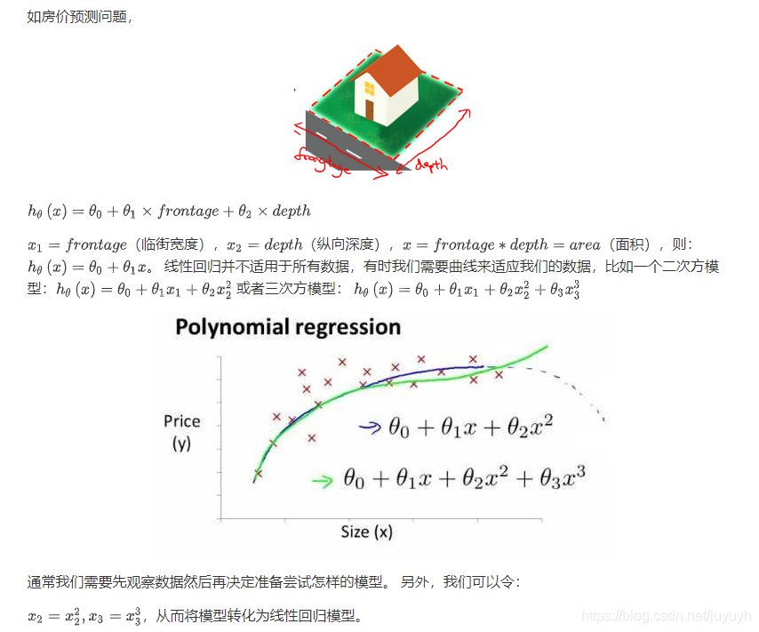
注：如果我们采用多项式回归模型，在运行梯度下降算法前，特征缩放非常有必要。

正规方程

theta = pinv(X'*X)*X'*y

对比:

梯度下降	正规方程
需要选择学习率	不需要
需要多次迭代	一次运算得出
当特征数量n大时也能较好适用	需要计算 $(X^{T}X)^{-1}$ 如果特征数量n较大则运算代价大，因为矩阵逆的计算时间复杂度为 $O(n^{3})$ ，通常来说当n小于10000 时还是可以接受的
适用于各种类型的模型	只适用于线性模型，不适合逻辑回归模型等其他模型

作业一

多变量线性回归作业答案

ex1_multi.m(price = [1 (([1650 3]-mu) ./ sigma)] * theta ;)

%% Machine Learning Online Class
%  Exercise 1: Linear regression with multiple variables
%
%  Instructions
%  ------------
% 
%  This file contains code that helps you get started on the
%  linear regression exercise. 
%
%  You will need to complete the following functions in this 
%  exericse:
%
%     warmUpExercise.m
%     plotData.m
%     gradientDescent.m
%     computeCost.m
%     gradientDescentMulti.m
%     computeCostMulti.m
%     featureNormalize.m
%     normalEqn.m
%
%  For this part of the exercise, you will need to change some
%  parts of the code below for various experiments (e.g., changing
%  learning rates).
%

%% Initialization

%% ================ Part 1: Feature Normalization ================

%% Clear and Close Figures
clear ; close all; clc

fprintf('Loading data ...\n');

%% Load Data
data = load('ex1data2.txt');
X = data(:, 1:2);
y = data(:, 3);
m = length(y);

% Print out some data points
fprintf('First 10 examples from the dataset: \n');
fprintf(' x = [%.0f %.0f], y = %.0f \n', [X(1:10,:) y(1:10,:)]');

fprintf('Program paused. Press enter to continue.\n');
pause;

% Scale features and set them to zero mean
fprintf('Normalizing Features ...\n');

[X mu sigma] = featureNormalize(X);      % 均值0，标准差1

% Add intercept term to X
X = [ones(m, 1) X];


%% ================ Part 2: Gradient Descent ================

% ====================== YOUR CODE HERE ======================
% Instructions: We have provided you with the following starter
%               code that runs gradient descent with a particular
%               learning rate (alpha). 
%
%               Your task is to first make sure that your functions - 
%               computeCost and gradientDescent already work with 
%               this starter code and support multiple variables.
%
%               After that, try running gradient descent with 
%               different values of alpha and see which one gives
%               you the best result.
%
%               Finally, you should complete the code at the end
%               to predict the price of a 1650 sq-ft, 3 br house.
%
% Hint: By using the 'hold on' command, you can plot multiple
%       graphs on the same figure.
%
% Hint: At prediction, make sure you do the same feature normalization.
%

fprintf('Running gradient descent ...\n');

% Choose some alpha value
alpha = 0.1;
num_iters = 50;

% Init Theta and Run Gradient Descent 
theta = zeros(3, 1);
[theta, J_history] = gradientDescentMulti(X, y, theta, alpha, num_iters);

% Plot the convergence graph
figure;
plot(1:numel(J_history), J_history, '-b', 'LineWidth', 2);
xlabel('Number of iterations');
ylabel('Cost J');

% Display gradient descent's result
fprintf('Theta computed from gradient descent: \n');
fprintf(' %f \n', theta);
fprintf('\n');

% Estimate the price of a 1650 sq-ft, 3 br house
% ====================== YOUR CODE HERE ======================
% Recall that the first column of X is all-ones. Thus, it does
% not need to be normalized.
price = [1 (([1650 3]-mu) ./ sigma)] * theta ;
% ============================================================

fprintf(['Predicted price of a 1650 sq-ft, 3 br house ' ...
         '(using gradient descent):\n $%f\n'], price);

fprintf('Program paused. Press enter to continue.\n');
pause;

%% ================ Part 3: Normal Equations ================

fprintf('Solving with normal equations...\n');

% ====================== YOUR CODE HERE ======================
% Instructions: The following code computes the closed form 
%               solution for linear regression using the normal
%               equations. You should complete the code in 
%               normalEqn.m
%
%               After doing so, you should complete this code 
%               to predict the price of a 1650 sq-ft, 3 br house.
%

%% Load Data
data = csvread('ex1data2.txt');
X = data(:, 1:2);
y = data(:, 3);
m = length(y);

% Add intercept term to X
X = [ones(m, 1) X];

% Calculate the parameters from the normal equation
theta = normalEqn(X, y);

% Display normal equation's result
fprintf('Theta computed from the normal equations: \n');
fprintf(' %f \n', theta);
fprintf('\n');


% Estimate the price of a 1650 sq-ft, 3 br house
% ====================== YOUR CODE HERE ======================
price = [1 1650 3] * theta ;


% ============================================================

fprintf(['Predicted price of a 1650 sq-ft, 3 br house ' ...
         '(using normal equations):\n $%f\n'], price);

特征值缩放( $x_{n} = \frac{x_{n}-\mu _{n}}{s_{n}}$ )

function [X_norm, mu, sigma] = featureNormalize(X)

% You need to set these values correctly
X_norm = X;
mu = zeros(1, size(X, 2));
sigma = zeros(1, size(X, 2));
       
mu(1) = mean(X_norm(:,1));
mu(2) = mean(X_norm(:,2));

sigma(1) = std(X_norm(:,1));
sigma(2) = std(X_norm(:,2));

X_norm(:,1) = (X_norm(:,1).-mu(1))/sigma(1);
X_norm(:,2) = (X_norm(:,2).-mu(2))/sigma(2);

end

代价函数( $J =\frac{(X\theta -y)^{T}(X\theta-y)}{2m}$ )分子等价 $\sum_{i}^{m}(h_{\theta }(x^{(i)})-y^{(i)})^{2}$

function J = computeCostMulti(X, y, theta)

m = length(y); % number of training examples

J = 0;

J = (X*theta-y)'*(X*theta-y)/(2*m);   

end

梯度下降( $\theta = \theta - \alpha (\frac{1}{m}((X\theta - y)^{T}X)^{T})$ )

function [theta, J_history] = gradientDescentMulti(X, y, theta, alpha, num_iters)

m = length(y); % number of training examples
J_history = zeros(num_iters, 1);

for iter = 1:num_iters
    theta = theta -alpha/m*((X*theta-y)'*X)';    
    J_history(iter) = computeCostMulti(X, y, theta);

end
J_history
end

正则方程( $\theta = (X^{T}X)^{-1}X^{T}y$ )

function [theta] = normalEqn(X, y)


theta = zeros(size(X, 2), 1);

theta = pinv(X'*X)*X'*y;

end

吴恩达 机器学习 (线性回归)

第一章: 引言

第二章: 单变量线性回归

第四章: 多变量线性回归

吴恩达机器学习 (线性回归)