python 时间序列预测——LSTM, GRU

最新推荐文章于 2025-09-14 20:03:13 发布

原创最新推荐文章于 2025-09-14 20:03:13 发布 · 9.7k 阅读

103 ·

CC 4.0 BY-SA版权

我们不生产知识，我们只是互联网的搬运工

编程语言同时被 2 个专栏收录

240 篇文章

订阅专栏

时间序列

90 篇文章

订阅专栏

本文通过使用长短期记忆网络（LSTM）和门控循环单元（GRU）两种深度学习模型，对太阳黑子数据集进行时间序列预测。详细介绍了数据预处理、模型搭建、训练及评估过程。

数据集

太阳黑子数据集，Monthly Sunspots

下载

import numpy as np
import pandas as pd

url = "http://www.sidc.be/silso/INFO/snmtotcsv.php"
data = pd.read_csv (url,sep =";")
loc = "Monthly Sunspots.csv"
data . to_csv (loc , index = False )

data_csv = pd. read_csv (loc , header = None )
yt= data_csv . iloc [0:3210 ,3]
print(yt.head())
'''
0     96.7
1    104.3
2    116.7
3     92.8
4    141.7
Name: 3, dtype: float64
'''
print(yt.tail())
'''
3205    56.4
3206    54.1
3207    37.9
3208    51.5
3209    20.5
Name: 3, dtype: float64
'''
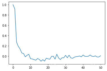
x_pacf=pacf(yt ,nlags=50, method='ols')
plt.plot(x_pacf)

该时间序列的 偏自相关函数【百度百科】
在这里插入图片描述

预处理

引入时滞

用紧邻的5个历史数据预测下一时刻

yt_1 =yt. shift (1)
yt_2 =yt. shift (2)
yt_3 =yt. shift (3)
yt_4 =yt. shift (4)
yt_5 =yt. shift (5)
data =pd. concat ([yt ,yt_1 , yt_2 ,yt_3 ,yt_4 ,yt_5 ], axis =1)
data . columns = ['yt', 'yt_1', 'yt_2', 'yt_3', 'yt_4', 'yt_5']
data = data . dropna ()  # 除去NULL，因为序列的起始点是没有历史的
print(data.tail( 6 ))
'''
        yt  yt_1  yt_2  yt_3  yt_4  yt_5
3204  57.0  58.0  62.2  63.6  78.6  64.4
3205  56.4  57.0  58.0  62.2  63.6  78.6
3206  54.1  56.4  57.0  58.0  62.2  63.6
3207  37.9  54.1  56.4  57.0  58.0  62.2
3208  51.5  37.9  54.1  56.4  57.0  58.0
3209  20.5  51.5  37.9  54.1  56.4  57.0
'''
print(data.head(6))
'''
       yt   yt_1   yt_2   yt_3   yt_4   yt_5
5   139.2  141.7   92.8  116.7  104.3   96.7
6   158.0  139.2  141.7   92.8  116.7  104.3
7   110.5  158.0  139.2  141.7   92.8  116.7
8   126.5  110.5  158.0  139.2  141.7   92.8
9   125.8  126.5  110.5  158.0  139.2  141.7
10  264.3  125.8  126.5  110.5  158.0  139.2
'''
y = data ['yt']
x = data ['yt_1', 'yt_2', 'yt_3', 'yt_4', 'yt_5']

归一化

scaler_x = preprocessing . MinMaxScaler (feature_range =(-1, 1))
x = np. array (x). reshape (( len(x) ,5 ))
x = scaler_x . fit_transform (x)
scaler_y = preprocessing . MinMaxScaler (
feature_range =( -1, 1))
y = np. array (y). reshape (( len(y), 1))
y = scaler_y . fit_transform (y)
train_end = 3042
x_train =x[0: train_end ,]
x_test =x[ train_end +1:3205 ,]
y_train =y[0: train_end ]
y_test =y[ train_end +1:3205]
x_train = x_train . reshape ( x_train . shape + (1 ,))
x_test = x_test . reshape ( x_test . shape + (1 ,))
print(x_train . shape)  # (3042, 5, 1)

LSTM

from keras . layers . recurrent import LSTM

seed =2019
np.random.seed( seed )

model = Sequential()
model .add(LSTM (units =4, activation = 'tanh', recurrent_activation ='hard_sigmoid',input_shape = (5 , 1)))
model .add(Dense (units =1, activation = 'linear'))
model . compile ( loss ='mean_squared_error',optimizer = 'rmsprop')
model .fit( x_train , y_train , batch_size =1, epochs =10 , shuffle = True ) ## shuffle matters！！ 
print(model . summary ())
'''
_________________________________________________________________
Layer (type)                 Output Shape              Param #   
=================================================================
lstm_16 (LSTM)               (None, 4)                 96        
_________________________________________________________________
dense_64 (Dense)             (None, 1)                 5         
=================================================================
Total params: 101
Trainable params: 101
Non-trainable params: 0
_________________________________________________________________
None
'''

score_train = model.evaluate (x_train , y_train , batch_size =1)
score_test = model.evaluate (x_test , y_test , batch_size =1)
print ("in train MSE = ", round( score_train,4))
print ("in test MSE = ", round( score_test ,4))

pred = model.predict(x_test)
# pred1 = scaler_y.inverse_transform(np.array(pred1).reshape((len(pred1), 1)))

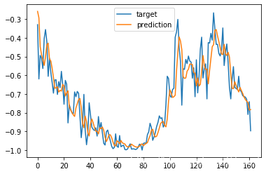
plt.plot(y_test)
plt.plot(pred)
plt.legend(['target','prediction'])

训练时 shuffle

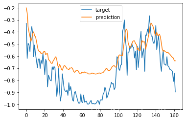
可以对比看看，不打乱数据集的训练效果会差一点。

打乱数据集：
在这里插入图片描述
不打乱数据集：

GRU

from keras . layers . recurrent import GRU

seed =2019
np. random . seed ( seed )
model = Sequential ()
model .add(GRU(units=4,
                return_sequences =False ,
                activation ='tanh', 
                recurrent_activation ='hard_sigmoid',
                input_shape =(5 , 1)))
model .add(Dense(units =1, activation ='linear'))
model . compile (loss ='mean_squared_error',optimizer ='rmsprop')
print(model . summary ())
'''
_________________________________________________________________
Layer (type)                 Output Shape              Param #   
=================================================================
gru_8 (GRU)                  (None, 4)                 72        
_________________________________________________________________
dense_23 (Dense)             (None, 1)                 5         
=================================================================
Total params: 77
Trainable params: 77
Non-trainable params: 0
_________________________________________________________________
None
'''
model .fit( x_train , y_train , batch_size =1,epochs =10)

score_train = model . evaluate ( x_train ,y_train , batch_size =1)
score_test = model . evaluate (x_test , y_test , batch_size =1)
print ("in train MSE = ", round( score_train,5))
print ("in test MSE = ", round( score_test ,5))

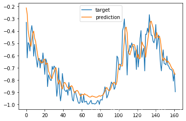
pred1 = model . predict ( x_test )
# pred1 = scaler_y .inverse_transform (np. array(pred1).reshape((len(pred1), 1)))

plt.plot(y_test)
plt.plot(pred1)
plt.legend(['target','prediction'])