科学计算与Matlab笔记：第4章：Matlab绘图

1. 二维曲线

plot函数&fplot函数

Plot函数

(1)plot函数的基本用法

plot（x,y）

其中，x与y分别用于存储x坐标与y坐标数据

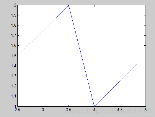
例1：绘制一条折线

>> x = [2.5, 3.5, 4, 5];
>> y=[1.5, 2.0, 1, 1.5];
>> plot(x,y)

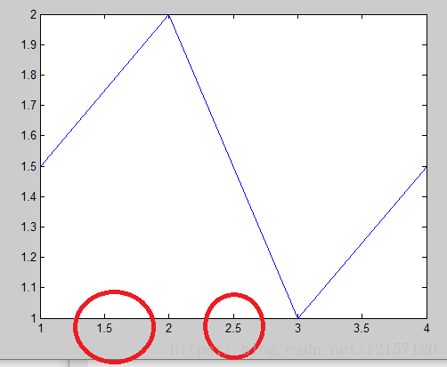
（2）最简单的plot函数调用方式

>> x=[1.5, 2.0, 1, 1.5];
>> plot(x)

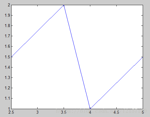
当plot函数的参数x是复数向量时，则分别以该向量元素实部与虚部为横纵坐标绘制一条曲线

>> x = [2.5, 3.5, 4, 5];
>> y=[1.5, 2.0, 1, 1.5];
>> cx = x + y*i;    //cx = complex（x，y）
>> plot(cx)

（3）plot（x，y）函数参数的变化形式

- 当x是向量，y是矩阵时

如果矩阵y的列数等于向量x的长度，则以向量x为横坐标，y的每个行向量为纵坐标绘制曲线，曲线的条数等于y的行数

如果矩阵y的行数等于向量x的长度，则以向量x为横坐标，y的每个列向量为纵坐标绘制曲线，曲线的条数等于y的列数

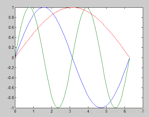
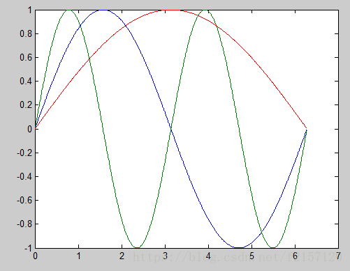
例2：绘制sin（x），sin（2x），sin（0.5x）的曲线

>> x = linspace(0,2*pi,100);
>> y = [sin(x);sin(2*x);sin(0.5*x)];
>> plot(x,y)

-当x，也是同型矩阵时

则以x，y对应列元素为横纵坐标分别绘制曲线，曲线条数等于矩阵的列数

>> t = 0:0.01:2*pi;
>> t1 = t';
>> x = [t1, t1, t1];
>> y = [sin(t1),sin(2*t1),sin(0.5*t1)];
>> plot(x,y)

（4）含多个输入参数的plot函数

plot(x1,y1,x2,y2,...,xn,yn)

其中每一向量构成一组数据点的横纵坐标，绘制一条曲线

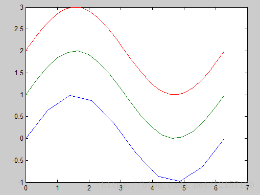
例3 采用不同数据点绘制正弦曲线，观察曲线的形态

>> t1 = linspace(0,2*pi,10);
>> t2 = linspace(0,2*pi,20);
>> t3 = linspace(0,2*pi,100);
>> plot(t1,sin(t1),t2,sin(t2)+1,t3,sin(t3)+2)

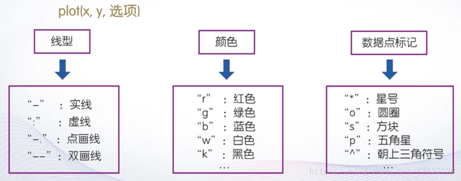
（5）含选项的plot函数

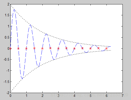
例4：用不同线形和颜色在同一坐标内绘制曲线y=2exp（-0.5x）*sin(2*pi*x)及其包络线

>> x=(0:pi/50:2*pi)';
>> y1 = 2*exp(-0.5*x)*[1,-1];
>> y2 = 2*exp(-0.5*x).*sin(2*pi*x);
>> x1 = 0:0.5:6;
>> y3 = 2*exp(-0.5*x1).*sin(2*pi*x1);
>> plot(x,y1,'k:',x,y2,'b--',x1,y3,'rp')

fplot函数

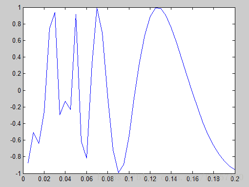
例5：绘制sin（1/x）的图形

>> x = 0:0.005:0.2;
>> y=sin(1./x);
>> plot(x,y)

（1）fplot函数基本用法

fplot(f,lims,选项)

其中，f代表一个函数，通常采用函数句柄的形式，lims为x轴的取值范围，用二元向量（xmin，xmax）描述，默认值为【-5，5】，选项定义与plot函数相同

例6：用fplot绘制sin（1/x）的图形

>> fplot(@(x)sin(1./x),[0,0.2],'b')

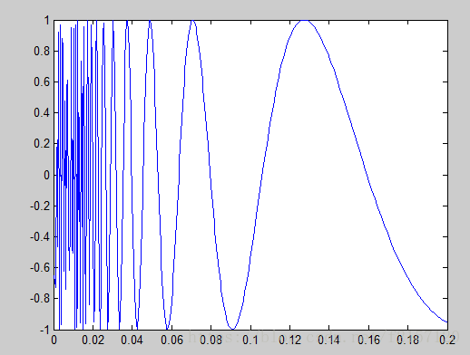
相比较plot函数，fplot会自动缩放坐标轴，避免丢失剧烈变化的细节信息。

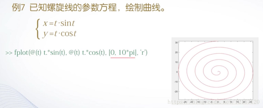
（2)双输入函数参数的用法

fplots（funx，funy，tlims，选项）

其中，funx，funy代表函数，通常采用函数句柄的形式，tlims为参数funx，funy的自变量的取值范围，用二元向量[tmin,tmax]描述

2.绘制图形的辅助操作

给图形添加标注

坐标控制

图形保持

图形窗口的分割

> Title(图形标题)

> xlable（x轴说明）

> ylable（y轴说明）

> text（x，y图例说明）

> legend（图例1，图例2，……）

（1）title函数

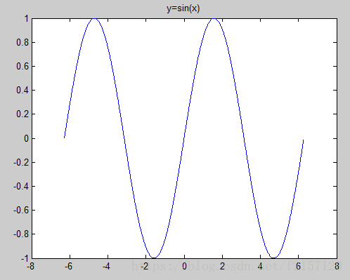
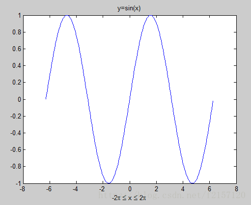
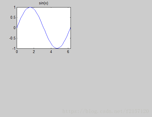
例1 绘制[-2pi, 2pi]区间的正弦曲线并给图形添加标题

>> x=-2*pi:0.01:2*pi;

>> y=sin(x);

>> plot(x,y)

>> title('y=sin(x)')

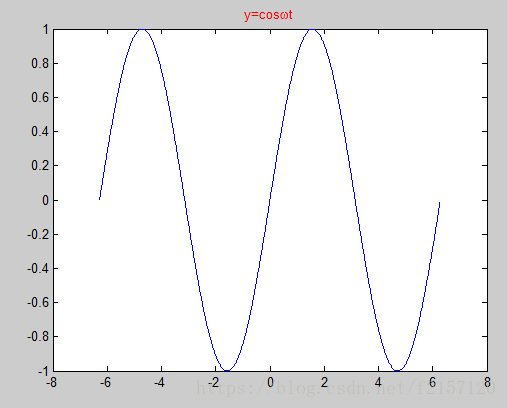
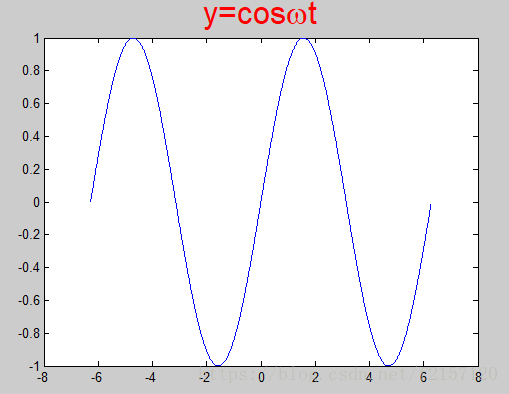
在图形标题中使用LaTeX格式控制符

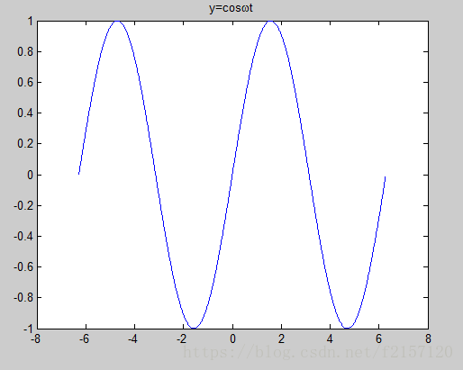
>> title('y=cos{\omega}t')

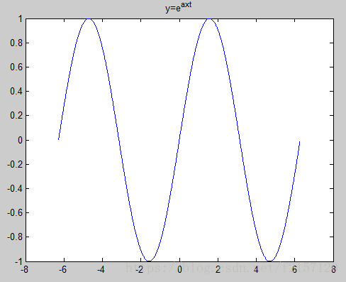
>> title('y=e^{axt}')

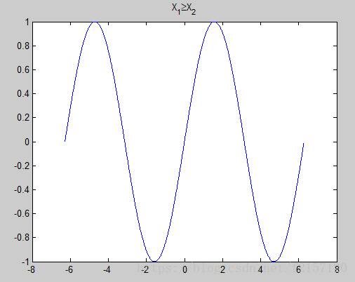
>> title('X_{1}{\geq}X_{2}')

>> title('{\bf y=cos{\omega}t +{\beta}}')

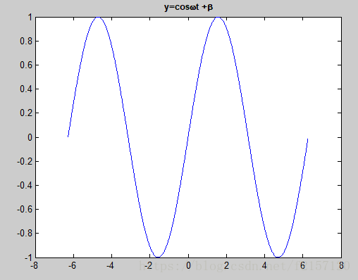
“\bf”: 加粗

“\it”：斜体

“\rm”：正体

含属性设置的title函数

Title(图形标题，属性名，属性值)

> color属性：用于设置图形标题文本的颜色

>>title('y=cos{\omega}t','Color','r')

> FontSize属性：用于设置标题文字的字号/默认字号为11

title('y=cos{\omega}t','FontSize',24)

（2）xlabel函数和ylabel函数

Xlabel(x轴说明)

ylabel(y轴说明)

>> x = -2*pi:0.05:2*pi;

>> y = sin(x);

>> plot(x,y)

>> title('y=sin(x)')

>> xlabel('-2\pi \leq x \leq 2\pi')

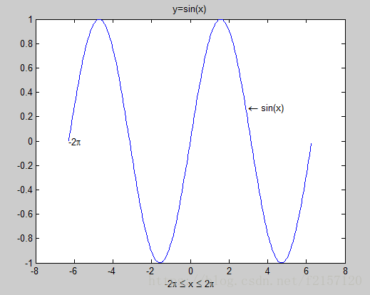
（3）text函数和gtext函数

Text（x,y,说明）

Gtext（说明）

>> text(-2*pi, 0,'-2{\pi}')

>> text(3, 0.28,'\leftarrow sin(x)')

（4）legend函数

Legend（图例1，图例2，……）

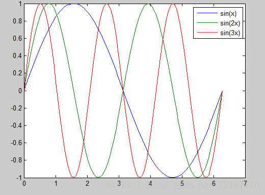
例2 绘制不同频率的正弦曲线，并用图例标出曲线。

>> x = linspace(0,2*pi,100);

>> plot(x,[sin(x);sin(2*x);sin(3*x)])

>>legend('sin(x)','sin(2x)','sin(3x)')

坐标控制

(1)axis函数

Axis的其他用法

Axis equal: 横、纵坐标采用等长刻度

Axis square：产生正方形坐标系，默认为矩形

Axis auto：使用默认设置

Axis off：取消坐标轴

Axis on：显示坐标轴

>> x = [0, 1, 1, 0, 0];

>> y = [0, 0, 1, 1, 0];

>> plot(x,y)

>> axis([-0.1, 1.1, -0.1, 1.1])

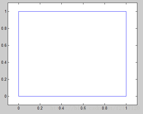
>> axis equal;

（2）给坐标加网格和边框

Grid on

Grid off

Grid 交互的打开，关闭网格

Box on

Box off

Box

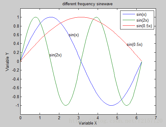
例3：绘制sin（x），sin（2x），sin（x/2）的函数曲线并添加图形标注

>>x=linspace(0,2*pi,100);

>> y=[sin(x);sin(2*x);sin(0.5*x)];

>> plot(x,y)

>> axis([0,7,-1.2,1.2])

>> title('different frequency sinewave');

>> xlabel('Variable X');

>> ylabel('Variable Y');

>> text(2.5,sin(2.5),'sin(x)');

>> text(1.5,sin(2*1.5),'sin(2x)');

>>text(5.5,sin(0.5*5.5),'sin(0.5x)');

>>legend('sin(x)','sin(2x)','sin(0.5x)');

>> grid on

 

图形保持

Hold on

Hold off

Hold

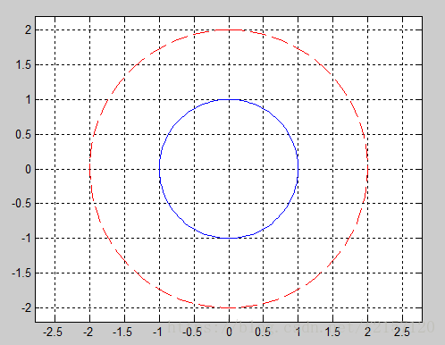
例4：用图形保持功能绘制两个同心圆

>> t=linspace(0,2*pi,100);

>> x=sin(t);

>> y=cos(t);

>> plot(x,y,'b')

>> hold on;

>> plot(2*x,2*y,'r--')

>> grid on

>> axis([-2.2,2.2,-2.2,2.2])

>> axis equal

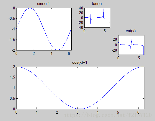
图形窗口的分割

子图：同一个图形窗口中不同坐标系下的图形

Subplot函数，subplot（m，n，p）

其中，m和n指定将图形窗口分成m x n个绘图区，p指定当前活动区 默认排序为按行排序。

>> subplot(2,2,1);

>> x=linspace(0,2*pi,60);

>> y=sin(x);

>> plot(x,y);

>> title('sin(x)');

>> axis([0,2*pi,-1,1]);

>> x=linspace(0,2*pi,60);

>> subplot(2,2,1);

>> plot(x,sin(x)-1);

>> title('sin(x)-1');

>> axis([0,2*pi,-2,0]);

>> subplot(2,1,2);

>> plot(x,cos(x)+1);

>> title('cos(x)+1');

>> axis([0,2*pi,0,2]);

>> subplot(4,4,3);

>> plot(x,tan(x));

>> title('tan(x)');

>> axis([0,2*pi,-40,40]);

>> subplot(4,4,8);

>> plot(x,cot(x));

>> title('cot(x)');

>> axis([0,2*pi,-35,35]);

>> 

3. 其它形式的二维图形

其它坐标系下的二维曲线

统计图

矢量图形

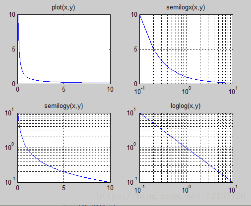
（1）对数坐标图

Semilogx（x1，y1，选项1，x2，y2，选项2，……）

Semilogy（x1，y1，选项1，x2，y2，选项2，……）

loglog（x1，y1，选项1，x2，y2，选项2，……）

例1：绘制1/x的直角线坐标图和三种对数坐标图

>>x=0:0.1:10;

>> y=1./x;

>> subplot(2,2,1);

>> plot(x,y);

>> title('plot(x,y)');

>> subplot(2,2,2);

>> semilogx(x,y)；

>> title('semilogx(x,y)');

>> grid on

>> subplot(2,2,3);

>> semilogy(x,y);

>> title('semilogy(x,y)');

>> grid on

>> subplot(2,2,4);

>> loglog(x,y);

>> title('loglog(x,y)');

>> grid on

>> 

（2）极坐标图

Polar（theta，rho，选项）

其中，theta为极角，rho为极径，选项的内容与plot函数相同

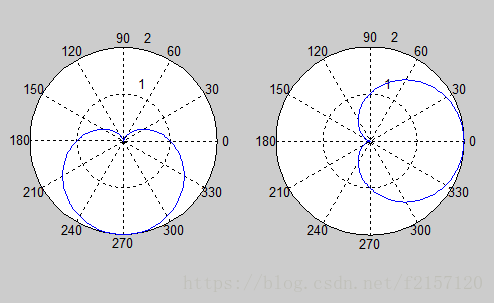
例2：按极坐标方程rho = 1-sin（theta）绘制心形曲线

>> t=0:pi/100:2*pi;

>> r=1-sin(t);

>> subplot(1,2,1);

>> polar(t,r);

>> subplot(1,2,2);

>> t1 = t-pi/2;

>> r1 = 1-sin(t1);

>> polar(t,r1)

统计图

条形图

直方图

饼图

散点图

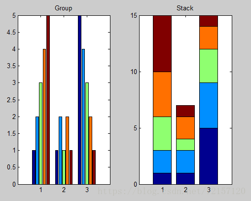
（1）条形类图形

条形图：bar函数，barh函数

Bar函数：bar（y，style）    “grouped”：簇状分组； “stacked”：堆积分组

其中，参数y是数据，选项style用于指定分组排列模式

例3：绘制分组条形图

>>y=[1,2,3,4,5;1,2,1,2,1;5,4,3,2,1];

>> subplot(1,2,1);

>> bar(y);

>> title('Group');

>> subplot(1,2,2);

>> bar(y,'stacked');

>> title('Stack');

>> y

y =

 

  1   2   3  4   5

  1   2   1  2   1

  5   4   3  2   1

 

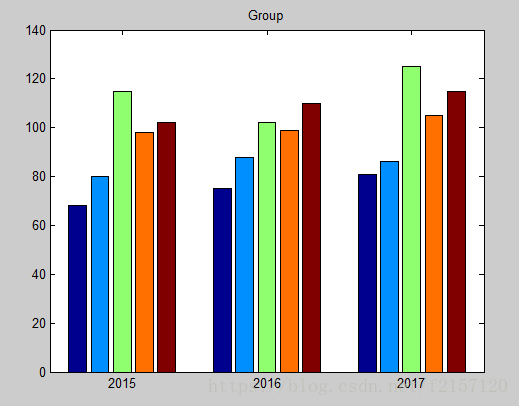
bar函数：bar（x，y，style），其中x存储横坐标，y存储数据

 >> x=[2015,2016,2017];

>> y=[68,80,115,98,102;75,88,102,99,110;81,86,125,105,115];

>> bar(x,y);

>> title('Group');

>> 

直方图：hist函数，rose函数

Hist函数：

hist（y）

hist（y，x）

其中，参数y是要统计的数据，x用于指定区间的划分方式

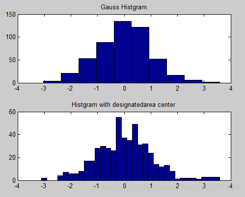
例5：绘制服从高斯分布的直方图

>>y=randn(500,1);

>> subplot(2,1,1);

>> hist(y);

>> title('Gauss Histgram');

>> subplot(2,1,2);

>> x=-3:0.2:3;

>> hist(y,x);

>> title('Histgram with designatedarea center');

>>

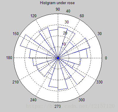
Rose函数：rose（theta，x）

其中，参数theta用于确定每一区间与原点的角度，选项x用于指定区间的划分方式

例6：绘制高斯分布数据在极坐标系下的直方图

>> y=randn(500,1);

>> theta=y*pi;

>> rose(theta);

>> title('Histgram under rose');

（2）面积类图形

Pie函数、area函数

Pie（x，explode）

其中，参数x存储待统计的数据，选项explode控制图块的显示方式

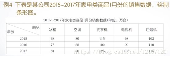
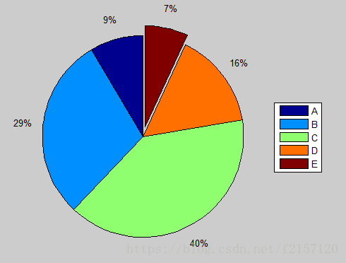
例7：某次考试优秀，良好，中等，及格，不及格的人数分别为：5,17,23,9,4，试用扇形统计图作成绩统计分析

>>score = [5,17,23,9,4];

>> ex = [0,0,0,0,1];

>> pie(score,ex)

>>legend('A','B','C','D','E','location','eastoutside')

>> 

 

（3）散点类图形

Scatter函数：散点图

Staris函数：阶梯图

Stem函数：杆图

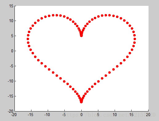
例8 以散点图的形式绘制桃心曲线，曲线的参数方程如下：

X=16sin^3(t)

Y=13cos(t)-5cos(2t)-2cos(3t)-cos(4t)

>> t = 0:pi/50:2*pi;

>> x=16*sin(t).^3;

>>y=13*cos(t)-5*cos(2*t)-2*cos(3*t)-cos(4*t);

>> scatter(x,y,'r','filled')

>> 

 

矢量类图形

Compass函数：罗盘图

Feather函数：羽毛图

Quiver函数：箭头图

Quiver函数的调用格式：quiver（x，y,u,v），其中，（x，y）指定矢量期间，（u，v）指定矢量终点

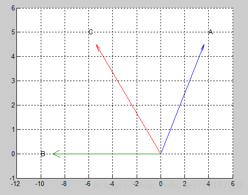
例9 已知向量A，B，求A+B，并用矢量图表示

>>A=[4,5];

>> B=[-10,0];

>> C=A+B;

>> hold on

>> quiver(0,0,A(1),A(2));

>> quiver(0,0,B(1),B(2));

>> quiver(0,0,C(1),C(2));

>> text(A(1),A(2),'A');

>> text(B(1),B(2),'B');

>> text(C(1),C(2),'C');

>> axis([-12,6,-1,6])

>> grid on

>> 

4.三维曲线

Plot3函数

Fplot3函数

（1）plot3函数的基本用法 plot3（x，y，z）

其中，参数x，y，z组成一组曲线的坐标

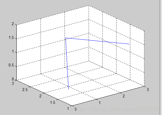
例1 绘制一条空间折线

>> x=[0.2,1.8,2.5];

>> y=[1.3,2.8,1.1];

>> z=[0.4,1.2,1.6];

>> plot3(x,y,z)

>> grid on

>> axis([0,3,1,3,0,2]);

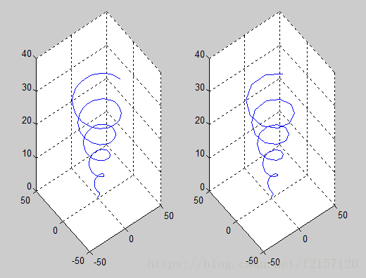
例2 绘制螺旋线x=sin(t) + t*cos(t);y=cos(t)-t*sin(t);z=t, (0 <= t <= 10*pi)

>> t=linspace(0,10*pi,200);

>> x=sin(t)+t.*cos(t);

>> y=cos(t)-t.*sin(t);

>> z=t;

>> subplot(1,2,1);

>> plot3(x,y,z);

>> grid on

>> subplot(1,2,2);

>> plot3(x(1:4:200),y(1:4:200),z(1:4:200));

>> grid on

>> 

(3)plot3函数参数的变化形式

Plot3（x，y，z）

参数x，y，z是同型矩阵

参数x，y，z中有向量，也有矩阵

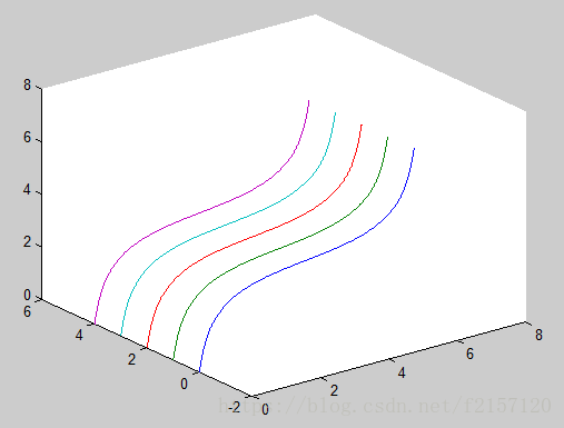
例3 在空间不同位置绘制5条正弦曲线

>> t = 0:0.01:2*pi;

>> t=t';

>> x=[t,t,t,t,t];

>>y=[sin(t),sin(t)+1,sin(t)+2,sin(t)+3,sin(t)+4];

>> z=[t,t,t,t,t];

>> plot3(x,y,z)

（3）含多组输入参数的plot3函数

Plot3(x1,y1,z1,x2,y2,z2,...,xn,yn,zn)

每一组x，y，z向量构成一组数据点的坐标，绘制一条曲线

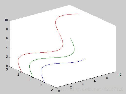
例4 绘制三条不同长度的正弦曲线

>>t = 0:0.01:1.5*pi;

>> t1 = 0:0.01:1.5*pi;

>> t2 = 0:0.01:2*pi;

>> t3 = 0:0.01:3*pi;

>>plot3(t1,sin(t1),t1,t2,sin(t2)+1,t2,t3,sin(t3)+2,t3)

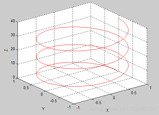
 例5 绘制空间曲线x=cos(t)；y=sin(t); z=2*t, (0 <= t <=6*pi)

>> t =0:pi/50:6*pi;

>> x=cos(t);

>> y=sin(t);

>> z=2*t;

>> plot3(x,y,z,'r');

>> xlabel('X');

>> ylabel('Y');

>> zlabel('Z');

>> grid on

Fplot3(funx,funy,funz,tlims)

其中，funx，funy，funz代表定义曲线x，y，z坐标的函数，通常采用函数句柄的形式。Tlims为参数函数自变量的取值范围，用二元向量[tmin, tmax]描述，默认为[-5, 5]

例6 绘制墨西哥帽顶曲线，曲线参数方程如下

X=exp(-t/10)*sin(5*t);

Y=exp(-t/10)*cos(5*t); [-12 <= t <=12]

Z=t;

>> xt = @(t)exp(-t/10).*sin(5*t);

>> yt = @(t)exp(-t/10).*cos(5*t);

>> zt = @(t)t;

>> fplot3(xt,yt,zt,[-12,12])

>> fplot3(xt,yt,zt,[-12,12],'r-')

 

5. 三维曲面

平面网格数据的生成

绘制三维曲面的mesh函数和surf函数

Fmesh函数和fsurf函数

平面网格数据的生成

（1）利用矩阵运算生成

>> x=2:6;

>> y=(3:8)';

>> X=ones(size(y))*x;

>> Y=y*ones(size(x));

（2）利用meshgrid函数生成

[X,Y]=meshgrid(x,y);

其中，参数x，y为向量，存储网格点坐标的X，Y为矩阵

>> x=2:6;

>> y=(3:8)';

>> [X,Y]=meshgrid(x,y);

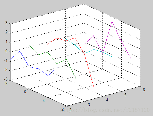
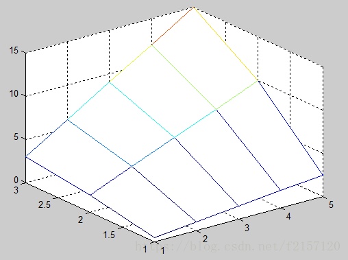
例1 绘制空间曲线

>> x=2:6;

>> y=(3:8)';

>> [X,Y]=meshgrid(x,y);

>> Z=randn(size(X));

>> plot3(X,Y,Z);

>> grid on

>> 

绘制三维曲面的函数

Mesh(x,y,z,c)

Surf(x,y,z,c)

其中，x，y是网格坐标矩阵，z是网格点上的高度矩阵，c用于指定在不同高度下的曲面颜色

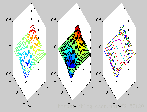
例2 绘制三维曲面图z=x*exp（-x^2 - y^2）

>> close all

>> t=-2:0.2:2;

>> [X,Y]=meshgrid(t);

>> Z=X.*exp(-X.^2-Y.^2);

>> subplot(1,3,1);

>> mesh(X,Y,Z);

>> subplot(1,3,2);

>> surf(X,Y,Z);

>> subplot(1,3,3);

>> plot3(X,Y,Z);

>> grid on

>> 

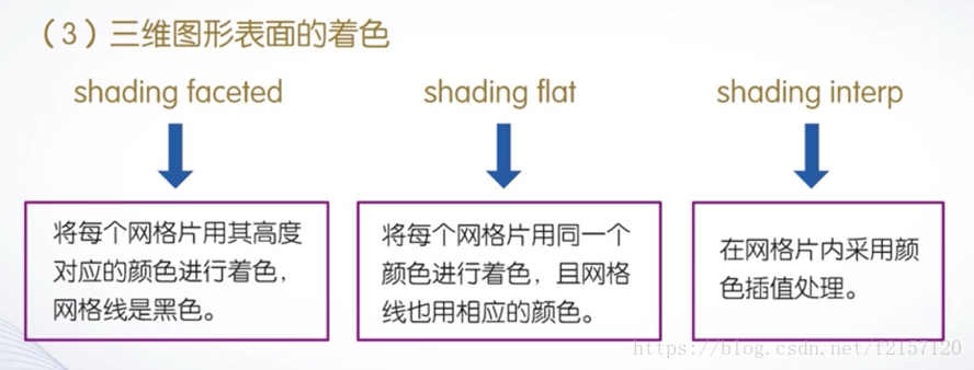
Mesh函数和surf函数的其他调用格式：

Mesh(z,c)

Surf(z,c)

当x，y省略时，z矩阵的第2维下标当作x轴坐标，z矩阵的第1维下标当作y轴坐标

>> t=1:5;

>> z=[0.5*t;2*t;3*t];

>> mesh(z);

绘制三维曲面的函数

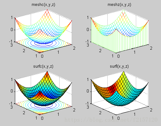
带等高线的三维网格曲面函数meshc

带底座的三维网格曲面函数meshz

具有等高线的曲面函数surfc

具有光照效果的曲面函数surfl

例3 用4种方法绘制函数z=（x-1)^2 +(y-2)^2 -1的曲面图，其中[0<= x <= 2],[1 <=y <= 3]

>> [x,y]=meshgrid(0:0.1:2,1:0.1:3);

>> z=(x-1).^2 + (y-2).^2 -1;

>> subplot(2,2,1);

>> meshc(x,y,z);

>> title('meshc(x,y,z)');

>> subplot(2,2,2);

>> meshz(x,y,z);

>> title('meshz(x,y,z)');

>> subplot(2,2,3);

>> surfc(x,y,z);

>> title('surfc(x,y,z)');

>> subplot(2,2,4);

>> surfl(x,y,z);

>> title('surfl(x,y,z)');

标准三维曲面

（1）sphere函数

[x,y,z]=sphere(n)

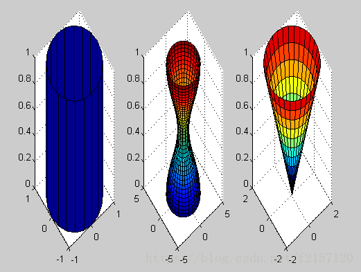
(2)cylinder函数

[x,y,z]=cylinder(R,n)

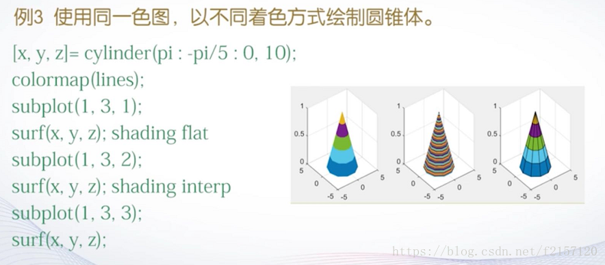
例4 用cylinder函数分别绘制柱面，花瓶和圆锥面

>> subplot(1,3,1);

>> [x,y,z]=cylinder;

>> surf(x,y,z);

>> subplot(1,3,2);

>> t=linspace(0,2*pi,40);

>> [x,y,z]=cylinder(2+cos(t),30);

>> surf(x,y,z);

>> subplot(1,3,3);

>> [x,y,z]=cylinder(0:0.2:2,30);

>> surf(x,y,z);

>> 

 

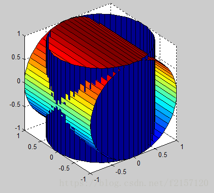
例5 用cylinder函数绘制两个相互垂直且直径相等的圆柱面的相交图形

>> [x,y,z]=cylinder(1,60);

>> z=[-1*z(2,:);z(2,:)];

>>surf(x,y,z);

>>hold on

>>surf(y,z,x);

>>axis equal

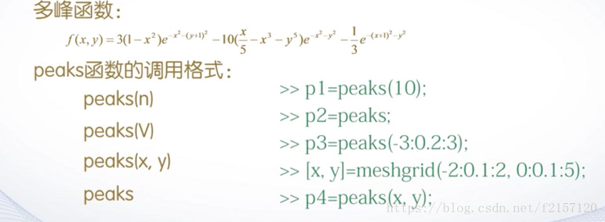
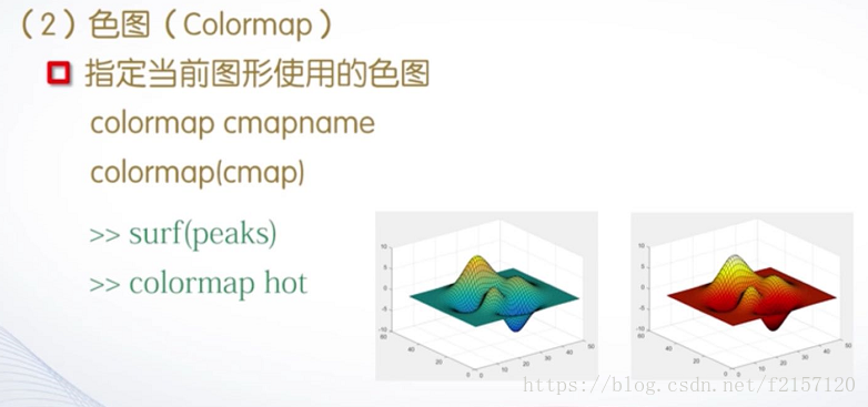
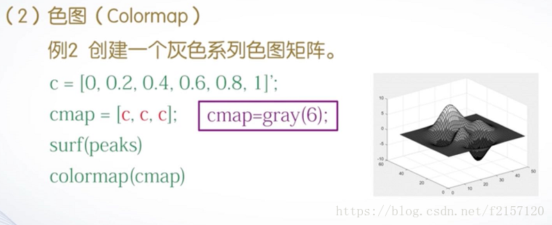
(3)peaks函数

多峰函数

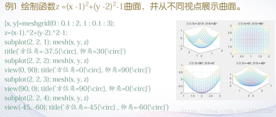
6， 图形的修饰处理

视点处理

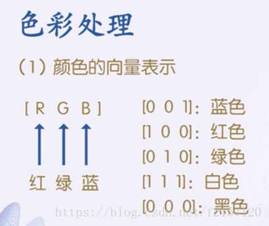
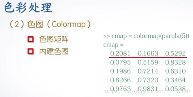
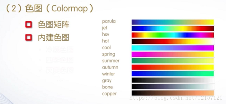
色彩处理

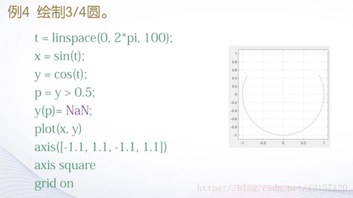
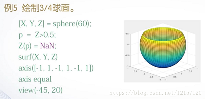
裁剪处理

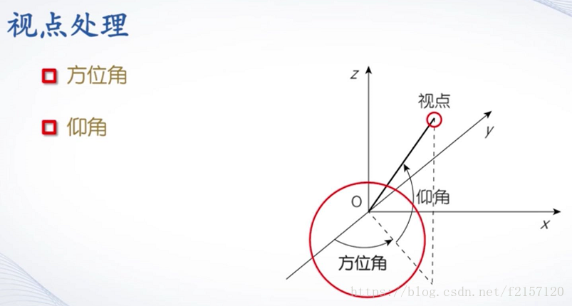
（1）view函数的基本用法

view（az，el）

其中，az为方位角，el为仰角

（2）view函数的其它用法

view(x,y,z)

view(2)

view(3)