Anomaly detection - Anomaly detection using the multivariate Gaussian distribution

最新推荐文章于 2024-03-24 17:38:58 发布

原创最新推荐文章于 2024-03-24 17:38:58 发布 · 214 阅读

0 ·

CC 4.0 BY-SA版权

人工智能同时被 2 个专栏收录

142 篇文章

订阅专栏

机器学习

109 篇文章

订阅专栏

本文深入探讨了一种基于多元高斯分布的异常检测算法。首先介绍了参数拟合过程，通过计算所有样例的平均值作为μ，估计协方差矩阵Σ。然后在训练集上构建模型，并对新测试样本计算其在高斯分布中的概率密度。如果概率低于阈值，则标记为异常。相较于原模型，多元高斯模型更能捕捉特征间的相关性。当Σ不可逆时，可能因特征冗余导致。最后，讨论了两种模型的适用场景，多元高斯模型适用于处理特征相关性的场景。

Let's develop a different anomaly detection algorithm based on multivariate Gaussian distribution.

Parameters fitting

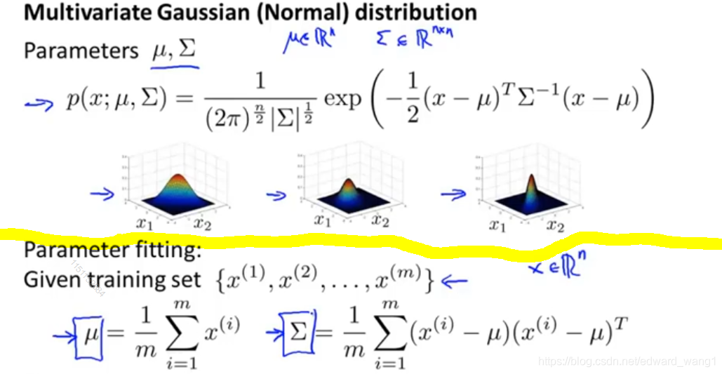
The upper part of figure-1 is a recap for definition of multivariate Gaussian distribution. Also it shows a range of different distributions as verying $\mu$ and $\Sigma$ . The lower part shows how to fit the parameters. If I have a set of examples

${x^{(1)}, x^{(2)},...,x^{(m)}}, x\in \mathbb{R}^{n}$

Then you set $\mu$ as the average of all examples. And set $\Sigma=\frac{1}{m}\sum _{i=1}^{m}(x^{(i)}-\mu )(x^{(i)}-\mu )^{T}$

So given the data set, we can estimate $\mu$ and $\Sigma$ . And get definition of $p(x; \mu , \Sigma )$

Multivariate Gaussian algorithm

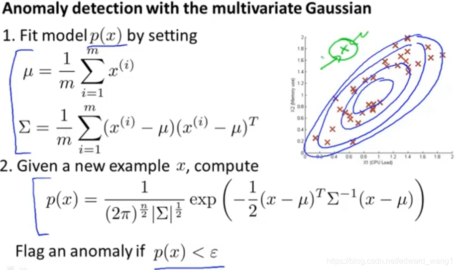
Figure-2 shows the steps of anomaly detection with multivariate Gaussian algorithm.

First, we take our training set and fit the model $p(x)$ by setting $\mu$ and $\Sigma$ as described in section "Parameters fitting".
Next, when you're given a new test example $x$ , the green cross, we need compute $p(x)$ using the formula for the multivariate Gaussian distribution.
Then, if $p(x)< \epsilon$ , we flag it as an anomaly; otherwise, we don't flag it as an anomaly.

It turns out, if we were to fit a multivariate Gaussain distribution to this data set (red crosses), you end up with a distribution that places lots of probability in the central regions, slightly less probability in the outer regions. And very low probability at the green cross point. And the green cross example will be correctly flaged as an anomaly.

Relationship to original model

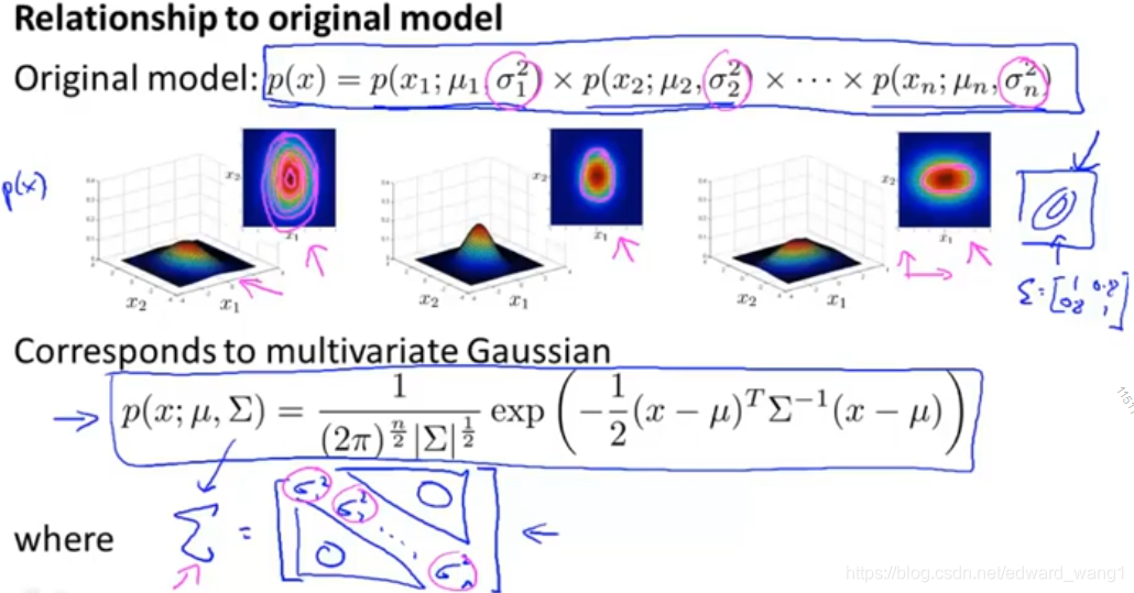
The original model corresponds to multivariate Gaussian where the contours of the Gaussian are always axes aligned.

Mathematically, it turns out that the original model

$p(x)=p(x_{1}; \mu _{1}, \sigma _{1}^{2}) \times p(x_{2}; \mu _{2}, \sigma _{2}^{2}) \times...\times p(x_{n}; \mu _{n}, \sigma _{n}^{2})$

is actually the same as a multivariate Gaussian distribution but with a constraint that everything on the off diagonal of $\Sigma$ is 0:

$\Sigma =\begin{bmatrix} \sigma _{1}^{2} & 0 & 0 & 0\\ 0 & \sigma _{2}^{2} & 0 & 0\\ 0 & 0 & ... & 0\\ 0 & 0 & 0 & \sigma _{n}^{2}\\ \end{bmatrix}$

if you plug $\sigma _{1}^{2}, \sigma _{2}^{2}...\sigma _{n}^{2}$ of original model into $\Sigma$ , then the two models are actually identical.

So the original model is actually a special case of this multivariate Gaussian model.

Which one to use?

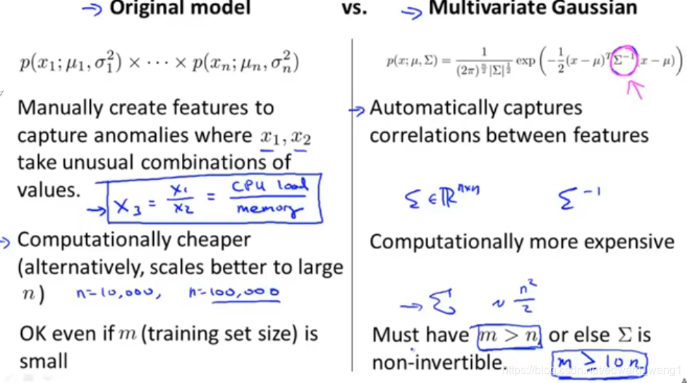
When would you use each of these two models? In general, the original model is probably used somewhat more often; whereas the multivariate Gaussian distribution is used somewhat less but it has the advantage of being able to capture correlations between features. Above figure-4 shows the scenarios.

If the sigma is singular

If you're fitting with multivariate Gaussian and find that $\Sigma$ is non-invertible, then there are usually two cases for this:

Failed to satisfy $m> n$ condition
You have redundant features which means that features that are linearly dependent. For example, you had two copies of the same feature; or maybe you have some feature like $x_{3}=x_{4}+x_{5}$ .

<end>