logistic回归，逻辑回归代码实现

我们将建立一个逻辑回归模型来预测一个学生是否被大学录取。假设你是一个大学系的管理员，你想根据两次考试的结果来决定每个申请人的录取机会。你有以前的申请人的历史数据，你可以用它作为逻辑回归的训练集。对于每一个培训例子，你有两个考试的申请人的分数和录取决定。为了做到这一点，我们将建立一个分类模型，根据考试成绩估计入学概率。

1.数据集：下载链接: https://pan.baidu.com/s/1IHqaJqDkSJ--igVV7kDsrg 密码: 2jbg

                 源码链接: https://pan.baidu.com/s/1uk2_zfaJH29SnU8buvyOwg 密码: k9vd

2.代码：

#三大件
import numpy as np
import pandas as pd
import matplotlib.pyplot as plt
%matplotlib inline

import os   #输出数据的前五行
path = 'data' + os.sep + 'LogiReg_data.txt'
pdData = pd.read_csv(path, header=None, names=['Exam 1', 'Exam 2', 'Admitted'])
pdData.head()

#用点图显示数据

positive = pdData[pdData['Admitted'] == 1] # returns the subset of rows such Admitted = 1, i.e. the set of *positive* examples

negative = pdData[pdData['Admitted'] == 0] # returns the subset of rows such Admitted = 0, i.e. the set of *negative* examples

fig, ax = plt.subplots(figsize=(10,5))
ax.scatter(positive['Exam 1'], positive['Exam 2'], s=30, c='b', marker='o', label='Admitted')
ax.scatter(negative['Exam 1'], negative['Exam 2'], s=30, c='r', marker='x', label='Not Admitted')
ax.legend()
ax.set_xlabel('Exam 1 Score')
ax.set_ylabel('Exam 2 Score')

plt.show()

The logistic regression

目标：建立分类器（求解出三个参数 θ0θ1θ2θ0θ1θ2）

设定阈值，根据阈值判断录取结果

要完成的模块

• sigmoid : 映射到概率的函数

• model : 返回预测结果值

• cost : 根据参数计算损失

• gradient : 计算每个参数的梯度方向

• descent : 进行参数更新

• accuracy: 计算精度

def sigmoid(z):   #定义sigmoid函数
    return 1 / (1 + np.exp(-z))

nums = np.arange(-10, 10, step=1) #显示sigmoid函数
fig, ax = plt.subplots(figsize=(12,4))
ax.plot(nums, sigmoid(nums), 'r')
plt.show()

def model(X, theta):
    
    return sigmoid(np.dot(X, theta.T))

pdData.insert(0, 'Ones', 1) # in a try / except structure so as not to return an error if the block si executed several times


# set X (training data) and y (target variable)
orig_data = pdData.as_matrix() # convert the Pandas representation of the data to an array useful for further computations
cols = orig_data.shape[1]
X = orig_data[:,0:cols-1]
y = orig_data[:,cols-1:cols]

# convert to numpy arrays and initalize the parameter array theta
#X = np.matrix(X.values)
#y = np.matrix(data.iloc[:,3:4].values) #np.array(y.values)
theta = np.zeros([1, 3])

损失函数

将对数似然函数去负号

D(hθ(x),y)=−ylog(hθ(x))−(1−y)log(1−hθ(x))
D(hθ(x),y)=−ylog⁡(hθ(x))−(1−y)log⁡(1−hθ(x))

求平均损失：

J(θ)=1n∑i=1nD(hθ(xi),yi)
J(θ)=1n∑i=1nD(hθ(xi),yi)

def cost(X, y, theta):  #计算平均损失
    left = np.multiply(-y, np.log(model(X, theta)))
    right = np.multiply(1 - y, np.log(1 - model(X, theta)))
    return np.sum(left - right) / (len(X)

计算梯度：

def gradient(X, y, theta):
    grad = np.zeros(theta.shape)
    error = (model(X, theta)- y).ravel()
    for j in range(len(theta.ravel())): #for each parmeter
        term = np.multiply(error, X[:,j])
        grad[0, j] = np.sum(term) / len(X)
    
    return grad

Gradient descent

比较3中不同梯度下降方法

STOP_ITER = 0
STOP_COST = 1
STOP_GRAD = 2

def stopCriterion(type, value, threshold):
    #设定三种不同的停止策略
    if type == STOP_ITER:        return value > threshold
    elif type == STOP_COST:      return abs(value[-1]-value[-2]) < threshold
    elif type == STOP_GRAD:      return np.linalg.norm(value) < threshold

import numpy.random
#洗牌
def shuffleData(data):
    np.random.shuffle(data)
    cols = data.shape[1]
    X = data[:, 0:cols-1]
    y = data[:, cols-1:]
    return X, y

def descent(data, theta, batchSize, stopType, thresh, alpha):
    #梯度下降求解
    
    init_time = time.time()
    i = 0 # 迭代次数
    k = 0 # batch
    X, y = shuffleData(data)
    grad = np.zeros(theta.shape) # 计算的梯度
    costs = [cost(X, y, theta)] # 损失值

    
    while True:
        grad = gradient(X[k:k+batchSize], y[k:k+batchSize], theta)
        k += batchSize #取batch数量个数据
        if k >= n: 
            k = 0 
            X, y = shuffleData(data) #重新洗牌
        theta = theta - alpha*grad # 参数更新
        costs.append(cost(X, y, theta)) # 计算新的损失
        i += 1 

        if stopType == STOP_ITER:       value = i
        elif stopType == STOP_COST:     value = costs
        elif stopType == STOP_GRAD:     value = grad
        if stopCriterion(stopType, value, thresh): break
    
    return theta, i-1, costs, grad, time.time() - init_time

def runExpe(data, theta, batchSize, stopType, thresh, alpha):
    #import pdb; pdb.set_trace();
    theta, iter, costs, grad, dur = descent(data, theta, batchSize, stopType, thresh, alpha)
    name = "Original" if (data[:,1]>2).sum() > 1 else "Scaled"
    name += " data - learning rate: {} - ".format(alpha)
    if batchSize==n: strDescType = "Gradient"
    elif batchSize==1:  strDescType = "Stochastic"
    else: strDescType = "Mini-batch ({})".format(batchSize)
    name += strDescType + " descent - Stop: "
    if stopType == STOP_ITER: strStop = "{} iterations".format(thresh)
    elif stopType == STOP_COST: strStop = "costs change < {}".format(thresh)
    else: strStop = "gradient norm < {}".format(thresh)
    name += strStop
    print ("***{}\nTheta: {} - Iter: {} - Last cost: {:03.2f} - Duration: {:03.2f}s".format(
        name, theta, iter, costs[-1], dur))
    fig, ax = plt.subplots(figsize=(12,4))
    ax.plot(np.arange(len(costs)), costs, 'r')
    ax.set_xlabel('Iterations')
    ax.set_ylabel('Cost')
    ax.set_title(name.upper() + ' - Error vs. Iteration')
    return theta

不同的停止策略

设定迭代次数

#选择的梯度下降方法是基于所有样本的
n=100
runExpe(orig_data, theta, n, STOP_ITER, thresh=5000, alpha=0.000001)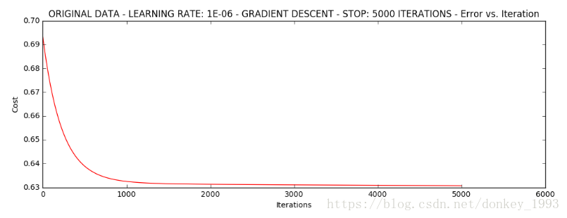

根据损失值停止

设定阈值 1E-6, 差不多需要110 000次迭代

runExpe(orig_data, theta, n, STOP_COST, thresh=0.000001, alpha=0.001)
plt.show()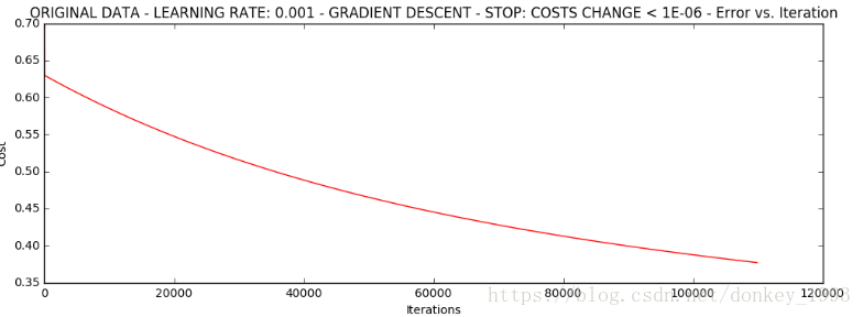

精度计算：

#设定阈值
def predict(X, theta):
    return [1 if x >= 0.5 else 0 for x in model(X, theta)]

scaled_X = scaled_data[:, :3]
y = scaled_data[:, 3]
predictions = predict(scaled_X, theta)
correct = [1 if ((a == 1 and b == 1) or (a == 0 and b == 0)) else 0 for (a, b) in zip(predictions, y)]
accuracy = (sum(map(int, correct)) % len(correct))
print ('accuracy = {0}%'.format(accuracy))