【案例共创】基于华为开发者空间的RestNet50目标检测

原创于 2025-12-18 22:00:00 发布 · 493 阅读

4 ·

CC 4.0 BY-SA版权

文章标签：

#华为 #目标检测 #人工智能 #华为开发者空间

人工智能同时被 3 个专栏收录

280 篇文章

订阅专栏

华为开发者空间

168 篇文章

订阅专栏

算法

3 篇文章

订阅专栏

最新案例动态，请查阅【案例共创】基于华为开发者空间的RestNet50目标检测。小伙伴们快来领取华为开发者空间进行实操吧！

本案例由：梅科尔工作室提供

1 概述

1.1 案例介绍

ResNet50模型是一种深度卷积神经网络，它使用残差模块和跳跃连接来缓解梯度消失问题。反向传播算法在ResNet模型中同样起着到头重要的作用，它可以计算ResNet模型中各个权重的梯度，并更新权重，从而优化模型性能。本案例使用到开发者空间----工作台/AI Notebook。

本案例选择医院的病例数据作为示例，并借助开发者空间工作台提供的免费AI Notebook编辑器进行本地编辑函数、轻松部署上云，直观地展示Notebook支持AI训练模型的开发与调试能力和实际应用开发中为开发者带来的便利。

通过实际操作，让大家深入了解如何利用 Notebook开发并部署一个梯度与反向传播算法。在这个过程中，大家将学习到从函数创建、模型训练到应用部署以及与 API集成等一系列关键步骤，从而掌握ResNet50的基本使用方法，体验其在Notebook开发中的优势。

1.2 适用对象

企业
个人开发者
高校学生

1.3 案例时间

本案例总时长预计120分钟。

1.4 案例流程

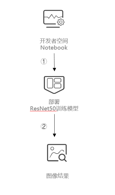
说明：

开发者空间进入Notebook；
在Notebook中用NPU训练模型，跑结果；

1.5 资源总览

| 资源名称 | 规格 | 单价（元） | 时长（分钟） |

| 开发者空间----工作台/AI Notebook | NPU basic · 1 * NPU 910B · 8v CPU · 24GB | 免费 | 120 |

2 梯度与反向传播算法

2.1 代码分析

环境配置

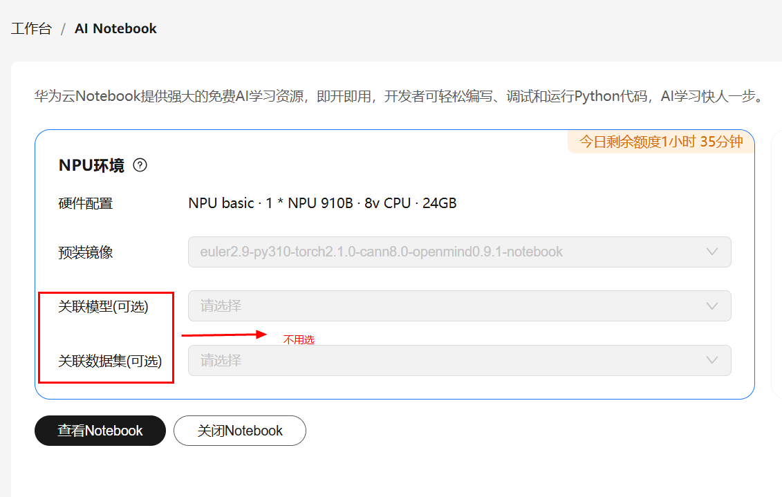
详细资源配置请参考案例华为开发者空间AI Notebook使用指导：步骤二。

进入华为开发者空间界面，进入AI Notebook页面。

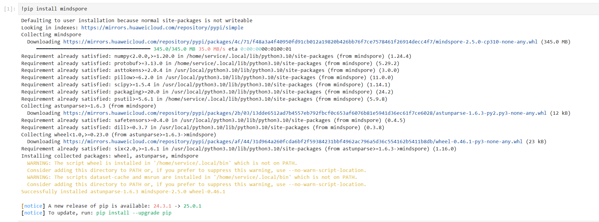
!pip install mindspore

!pip install numpy

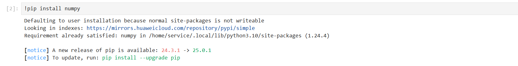
说明numpy模块已经被安装了。

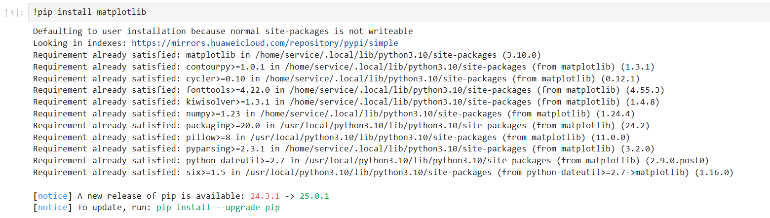
!pip install matplotlib

!pip install opencv-python

opencv模块在pip install安装失败，用-i指定其他下载源也安装失败，所以此处用yum install安装opencv模块。

!pip install pillow

MindSpore：深度学习框架，用于构建和训练模型。

NumPy：用于数值计算，处理数据。

Matplotlib：用于数据可视化，绘制图表。

OpenCV：用于图像处理，可能在数据预处理中使用。

Pillow：用于图像处理，加载和处理图像数据。

注：如果存在软件包下载失败，可以添加参数-i指定华为云的安装源。例如：

!pip install matplotlib -i https://repo.huaweicloud.com/repository/pypi/simple/

数据获取和准备

!wget <https://dtse-mirrors.obs.cn-north-4.myhuaweicloud.com/case/0036/skin-cancer-detection.tar>

!mkdir pifudata_Maker

!tar -xvf skin-cancer-detection.tar -C pifudata_Maker/

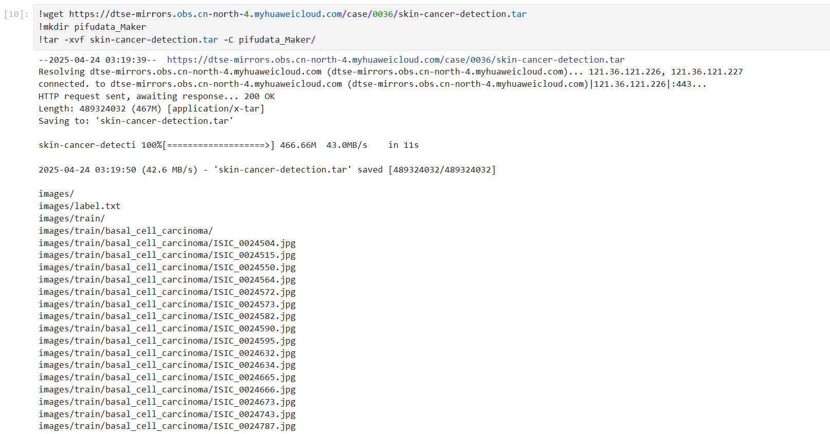
注释：使用git命令克隆数据集仓库，并解压数据集到指定文件夹。

分析：数据集是项目的基础，克隆和解压操作确保了数据的可用性。

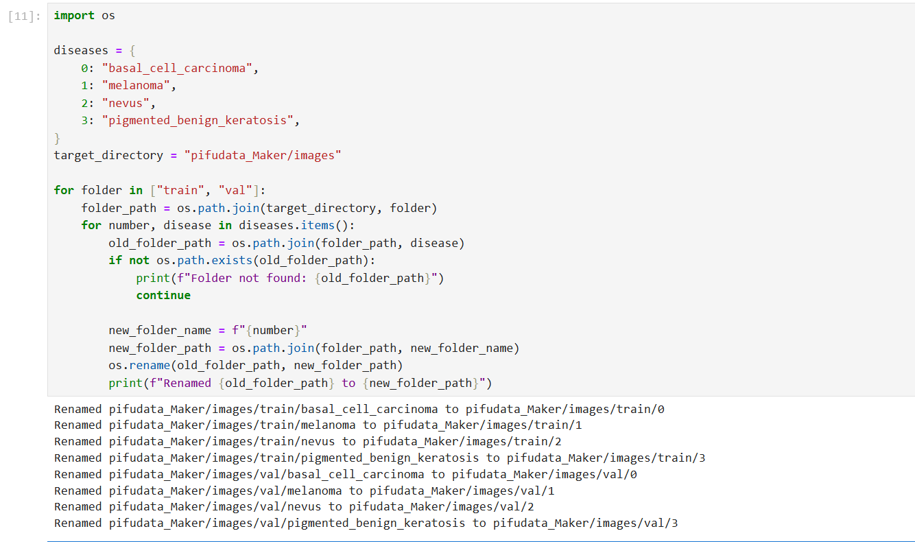
import os
diseases = {
0: "basal_cell_carcinoma",
1: "melanoma",
2: "nevus",
3: "pigmented_benign_keratosis",
}
target_directory = "pifudata_Maker/images"
for folder in ["train", "val"]:
folder_path = os.path.join(target_directory, folder)
for number, disease in diseases.items():
old_folder_path = os.path.join(folder_path, disease)
if not os.path.exists(old_folder_path):
print(f"Folder not found: {old_folder_path}")
continue
new_folder_name = f"{number}"
new_folder_path = os.path.join(folder_path, new_folder_name)
os.rename(old_folder_path, new_folder_path)
print(f"Renamed {old_folder_path} to {new_folder_path}")

注释：定义疾病名称和编号的映射，并对训练和验证数据集的文件夹进行重命名，方便后续处理。

分析：数据组织结构的调整有助于模型训练时的数据加载和管理。

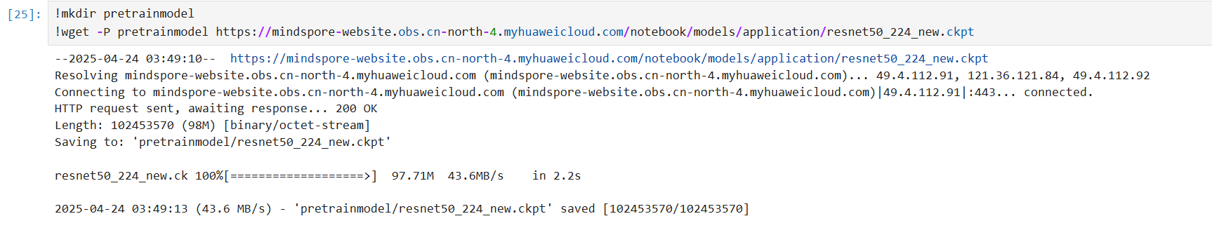
预训练模型准备

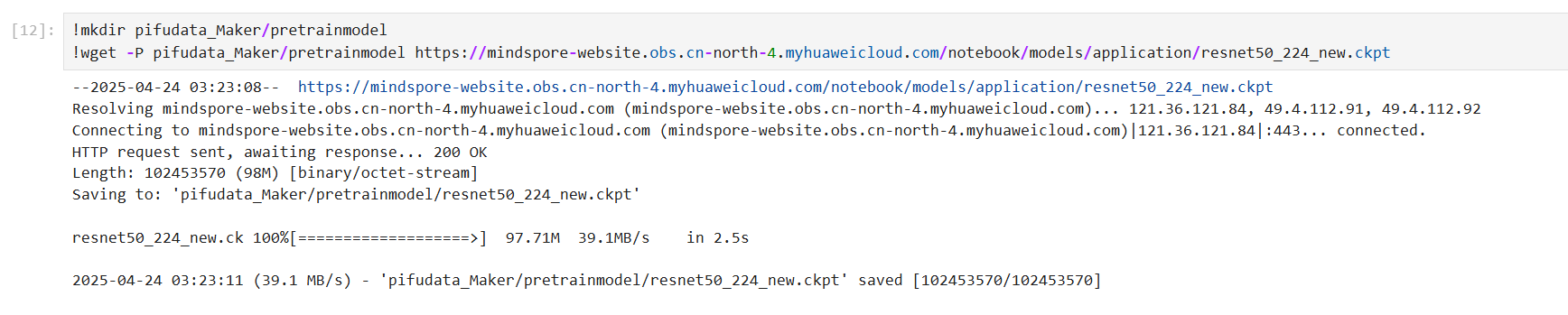
在工程文件下新建文件夹，命名为：pretrainmodel，然后在命令行中输入：

!mkdir pretrainmodel

!wget -P pretrainmodel <https://mindspore-website.obs.cn-north-4.myhuaweicloud.com/notebook/models/application/resnet50_224_new.ckpt>

注意：如果系统中没有wget环境请先安装：

sudo apt-get install wget

数据可视化

注意：下面Python代码中，data_path_train和data_path_val需要根据实际位置进行修改。

import os
import matplotlib.pyplot as plt
diseases = {
0: "basal_cell_carcinoma",
1: "melanoma",
2: "nevus",
3: "pigmented_benign_keratosis",
}
data_path_train = "pifudata_Maker/images/train"
data_path_val = "pifudata_Maker/images/val"
file_counts_train = {}
file_counts_val = {}
for folder_name in os.listdir(data_path_train):
folder_path = os.path.join(data_path_train, folder_name)
if os.path.isdir(folder_path):
count = len(os.listdir(folder_path))
file_counts_train[diseases.get(folder_name, folder_name)] = count
for folder_name in os.listdir(data_path_val):
folder_path = os.path.join(data_path_val, folder_name)
if os.path.isdir(folder_path):
count = len(os.listdir(folder_path))
file_counts_val[diseases.get(folder_name, folder_name)] = count
train_categories = list(file_counts_train.keys())
plt.figure(figsize=(12, 8))
train_bars = plt.bar(train_categories, file_counts_train.values(), width=0.4, color='blue', label='Train')
val_bars = plt.bar([train_categories.index(cat) + 0.4 for cat in train_categories], [file_counts_val.get(cat, 0) for cat in train_categories], width=0.4, color='green', label='Validation')
plt.legend()
plt.xlabel('labels')
plt.ylabel('Number of Images')
plt.title('Training and Validation Datasets')
train_list = [diseases[int(i)] for i in train_categories]
plt.xticks([train_categories.index(cat) + 0.2 for cat in train_categories], train_list, rotation=30, fontsize='small')
for i, (train_bar, val_bar) in enumerate(zip(train_bars, val_bars)):
train_height = train_bar.get_height()
val_height = val_bar.get_height() if val_bar else 0
plt.text(train_bar.get_x() + train_bar.get_width() / 2, train_height, '{}'.format(train_height), ha='center', va='bottom')
plt.text(val_bar.get_x() + val_bar.get_width() / 2, val_height, '{}'.format(val_height), ha='center', va='bottom') if val_bar else None
plt.show()

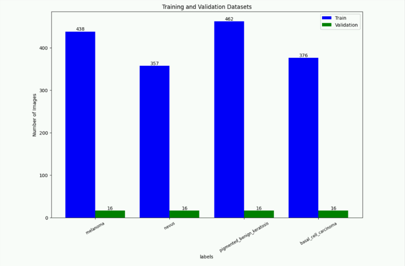
注释：统计训练和验证数据集中各类别的样本数量，并生成条形图进行可视化。

分析：数据分布的可视化有助于了解数据的平衡性，为模型训练提供参考。

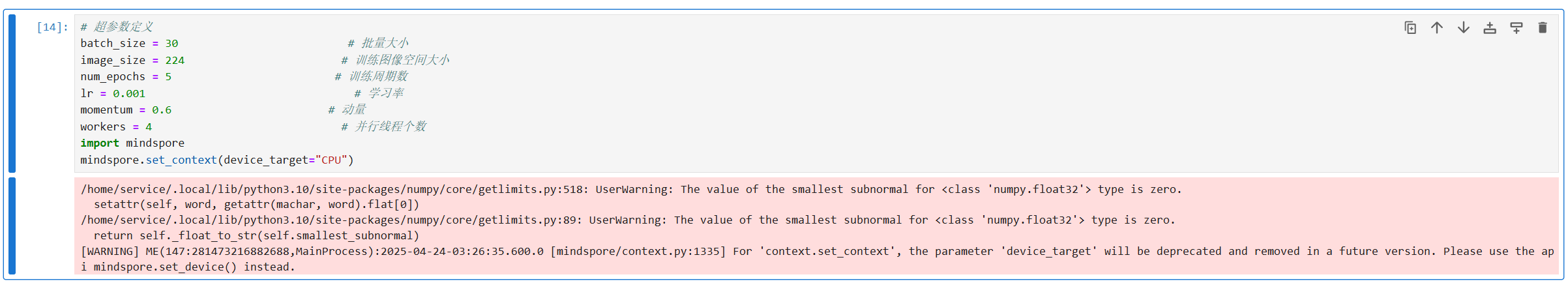
超参数定义

# 超参数定义
batch_size = 30 # 批量大小
image_size = 224 # 训练图像空间大小
num_epochs = 5 # 训练周期数
lr = 0.001 # 学习率
momentum = 0.6 # 动量
workers = 4 # 并行线程个数
import mindspore
mindspore.set_context(device_target="CPU")

注释：定义模型训练的超参数，包括批量大小、图像大小、训练周期数、学习率、动量和并行线程个数。

分析：超参数的选择对模型的训练效果和效率有重要影响，需要根据具体任务进行调整。

数据加载和预处理

import mindspore as ms
import mindspore.dataset as ds
import mindspore.dataset.vision as vision
# 数据集目录路径
data_path_train = "pifudata_Maker/images/train"
data_path_val = "pifudata_Maker/images/val"
# 创建训练数据集
def create_dataset_canidae(dataset_path, usage):
"""数据加载"""
data_set = ds.ImageFolderDataset(dataset_path,
num_parallel_workers=workers,
shuffle=True,)
# 数据增强操作
mean = [0.485 * 255, 0.456 * 255, 0.406 * 255]
std = [0.229 * 255, 0.224 * 255, 0.225 * 255]
scale = 32
if usage == "train":
# Define map operations for training dataset
trans = [
vision.RandomCropDecodeResize(size=image_size, scale=(0.08, 1.0), ratio=(0.75, 1.333)),
vision.RandomHorizontalFlip(prob=0.5),
vision.Normalize(mean=mean, std=std),
vision.HWC2CHW()
]
else:
# Define map operations for inference dataset
trans = [
vision.Decode(),
vision.Resize(image_size + scale),
vision.CenterCrop(image_size),
vision.Normalize(mean=mean, std=std),
vision.HWC2CHW()
]
# 数据映射操作
data_set = data_set.map(
operations=trans,
input_columns='image',
num_parallel_workers=workers)
# 批量操作
data_set = data_set.batch(batch_size)
return data_set
dataset_train = create_dataset_canidae(data_path_train, "train")
step_size_train = dataset_train.get_dataset_size()
dataset_val = create_dataset_canidae(data_path_val, "val")
step_size_val = dataset_val.get_dataset_size()
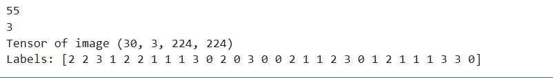
print(step_size_train)
print(step_size_val)
data = next(dataset_val.create_dict_iterator())
images = data["image"]
labels = data["label"]
# print(data["image"][0])
print("Tensor of image", images.shape)
print("Labels:", labels)

注释：定义数据加载和预处理函数，对训练和验证数据集进行不同的数据增强操作，并批量加载数据。

分析：数据增强可以提高模型的泛化能力，预处理操作确保输入数据的格式和分布符合模型的要求。

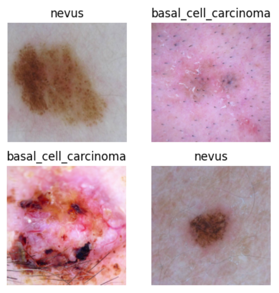
数据集可视化

import matplotlib.pyplot as plt
import numpy as np
# class_name对应label，按文件夹字符串从小到大的顺序标记label
class_name = {
0: "basal_cell_carcinoma",
1: "melanoma",
2: "nevus",
3: "pigmented_benign_keratosis",
}
# print(images[0])
plt.figure(figsize=(5, 5))
for i in range(4):
# 获取图像及其对应的label
# print(images[i])
data_image = images[i].asnumpy()
data_label = labels[i]
# 处理图像供展示使用
data_image = np.transpose(data_image, (1, 2, 0))
mean = np.array([0.485, 0.456, 0.406])
std = np.array([0.229, 0.224, 0.225])
data_image = std * data_image + mean
data_image = np.clip(data_image, 0, 1)
# 显示图像
plt.subplot(2, 2, i+1)
plt.imshow(data_image)
plt.title(class_name[int(labels[i].asnumpy())])
plt.axis("off")
plt.show()

注释：定义残差网络的基本模块、构建ResNet模型，并定义ResNet50的函数，支持加载预训练模型。

分析：ResNet模型通过残差连接解决了深度网络中的梯度消失问题，预训练模型的加载可以加速训练并提高模型性能。

**注意：**该部分Python代码最好与第5部分代码合在一起运行，以免报asnumpy()函数引用问题。

模型网络搭建

from typing import Type, Union, List, Optional
from mindspore import nn, train
from mindspore.common.initializer import Normal
weight_init = Normal(mean=0, sigma=0.02)
gamma_init = Normal(mean=1, sigma=0.02)
class ResidualBlockBase(nn.Cell):
expansion: int = 1 # 最后一个卷积核数量与第一个卷积核数量相等
def __init__(self, in_channel: int, out_channel: int,
stride: int = 1, norm: Optional[nn.Cell] = None,
down_sample: Optional[nn.Cell] = None) -> None:
super(ResidualBlockBase, self).__init__()
if not norm:
self.norm = nn.BatchNorm2d(out_channel)
else:
self.norm = norm
self.conv1 = nn.Conv2d(in_channel, out_channel,
kernel_size=3, stride=stride,
weight_init=weight_init)
self.conv2 = nn.Conv2d(in_channel, out_channel,
kernel_size=3, weight_init=weight_init)
self.relu = nn.ReLU()
self.down_sample = down_sample
def construct(self, x):
"""ResidualBlockBase construct."""
identity = x # shortcuts分支
out = self.conv1(x) # 主分支第一层：3*3卷积层
out = self.norm(out)
out = self.relu(out)
out = self.conv2(out) # 主分支第二层：3*3卷积层
out = self.norm(out)
if self.down_sample is not None:
identity = self.down_sample(x)
out += identity # 输出为主分支与shortcuts之和
out = self.relu(out)
return out
class ResidualBlock(nn.Cell):
expansion = 4 # 最后一个卷积核的数量是第一个卷积核数量的4倍
def __init__(self, in_channel: int, out_channel: int,
stride: int = 1, down_sample: Optional[nn.Cell] = None) -> None:
super(ResidualBlock, self).__init__()
self.conv1 = nn.Conv2d(in_channel, out_channel,
kernel_size=1, weight_init=weight_init)
self.norm1 = nn.BatchNorm2d(out_channel)
self.conv2 = nn.Conv2d(out_channel, out_channel,
kernel_size=3, stride=stride,
weight_init=weight_init)
self.norm2 = nn.BatchNorm2d(out_channel)
self.conv3 = nn.Conv2d(out_channel, out_channel * self.expansion,
kernel_size=1, weight_init=weight_init)
self.norm3 = nn.BatchNorm2d(out_channel * self.expansion)
self.relu = nn.ReLU()
self.down_sample = down_sample
def construct(self, x):
identity = x # shortscuts分支
out = self.conv1(x) # 主分支第一层：1*1卷积层
out = self.norm1(out)
out = self.relu(out)
out = self.conv2(out) # 主分支第二层：3*3卷积层
out = self.norm2(out)
out = self.relu(out)
out = self.conv3(out) # 主分支第三层：1*1卷积层
out = self.norm3(out)
if self.down_sample is not None:
identity = self.down_sample(x)
out += identity # 输出为主分支与shortcuts之和
out = self.relu(out)
return out
def make_layer(last_out_channel, block: Type[Union[ResidualBlockBase, ResidualBlock]],
channel: int, block_nums: int, stride: int = 1):
down_sample = None # shortcuts分支
if stride != 1 or last_out_channel != channel * block.expansion:
down_sample = nn.SequentialCell([
nn.Conv2d(last_out_channel, channel * block.expansion,
kernel_size=1, stride=stride, weight_init=weight_init),
nn.BatchNorm2d(channel * block.expansion, gamma_init=gamma_init)
])
layers = []
layers.append(block(last_out_channel, channel, stride=stride, down_sample=down_sample))
in_channel = channel * block.expansion
# 堆叠残差网络
for _ in range(1, block_nums):
layers.append(block(in_channel, channel))
return nn.SequentialCell(layers)
from mindspore import load_checkpoint, load_param_into_net
class ResNet(nn.Cell):
def __init__(self, block: Type[Union[ResidualBlockBase, ResidualBlock]],
layer_nums: List[int], num_classes: int, input_channel: int) -> None:
super(ResNet, self).__init__()
self.relu = nn.ReLU()
# 第一个卷积层，输入channel为3（彩色图像），输出channel为64
self.conv1 = nn.Conv2d(3, 64, kernel_size=7, stride=2, weight_init=weight_init)
self.norm = nn.BatchNorm2d(64)
# 最大池化层，缩小图片的尺寸
self.max_pool = nn.MaxPool2d(kernel_size=3, stride=2, pad_mode='same')
# 各个残差网络结构块定义，
self.layer1 = make_layer(64, block, 64, layer_nums[0])
self.layer2 = make_layer(64 * block.expansion, block, 128, layer_nums[1], stride=2)
self.layer3 = make_layer(128 * block.expansion, block, 256, layer_nums[2], stride=2)
self.layer4 = make_layer(256 * block.expansion, block, 512, layer_nums[3], stride=2)
# 平均池化层
self.avg_pool = nn.AvgPool2d()
# flattern层
self.flatten = nn.Flatten()
# 全连接层
self.fc = nn.Dense(in_channels=input_channel, out_channels=num_classes)
def construct(self, x):
x = self.conv1(x)
x = self.norm(x)
x = self.relu(x)
x = self.max_pool(x)
x = self.layer1(x)
x = self.layer2(x)
x = self.layer3(x)
x = self.layer4(x)
x = self.avg_pool(x)
x = self.flatten(x)
x = self.fc(x)
return x
def download_pretrained_model(url, save_path):
# 创建目录
os.makedirs(os.path.dirname(save_path), exist_ok=True)
# 下载文件
urllib.request.urlretrieve(url, save_path)
print(f"预训练模型已下载到: {save_path}")
def _resnet(model_url: str, block: Type[Union[ResidualBlockBase, ResidualBlock]],
layers: List[int], num_classes: int, pretrained: bool, pretrianed_ckpt: str,
input_channel: int):
model = ResNet(block, layers, num_classes, input_channel)
if pretrained:
# 加载预训练模型
# download(url=model_url, path=pretrianed_ckpt, replace=True)
param_dict = load_checkpoint(pretrianed_ckpt)
load_param_into_net(model, param_dict)
return model
def resnet50(num_classes: int = 1000, pretrained: bool = False):
"ResNet50模型"
resnet50_url = "https://mindspore-website.obs.cn-north-4.myhuaweicloud.com/notebook/models/application/resnet50_224_new.ckpt"
resnet50_ckpt = "./pretrainmodel/resnet50_224_new.ckpt"
return _resnet(resnet50_url, ResidualBlock, [3, 4, 6, 3], num_classes,
pretrained, resnet50_ckpt, 2048)

注释：定义残差网络的基本模块、构建ResNet模型，并定义ResNet50的函数，支持加载预训练模型。

分析：ResNet模型通过残差连接解决了深度网络中的梯度消失问题，预训练模型的加载可以加速训练并提高模型性能。

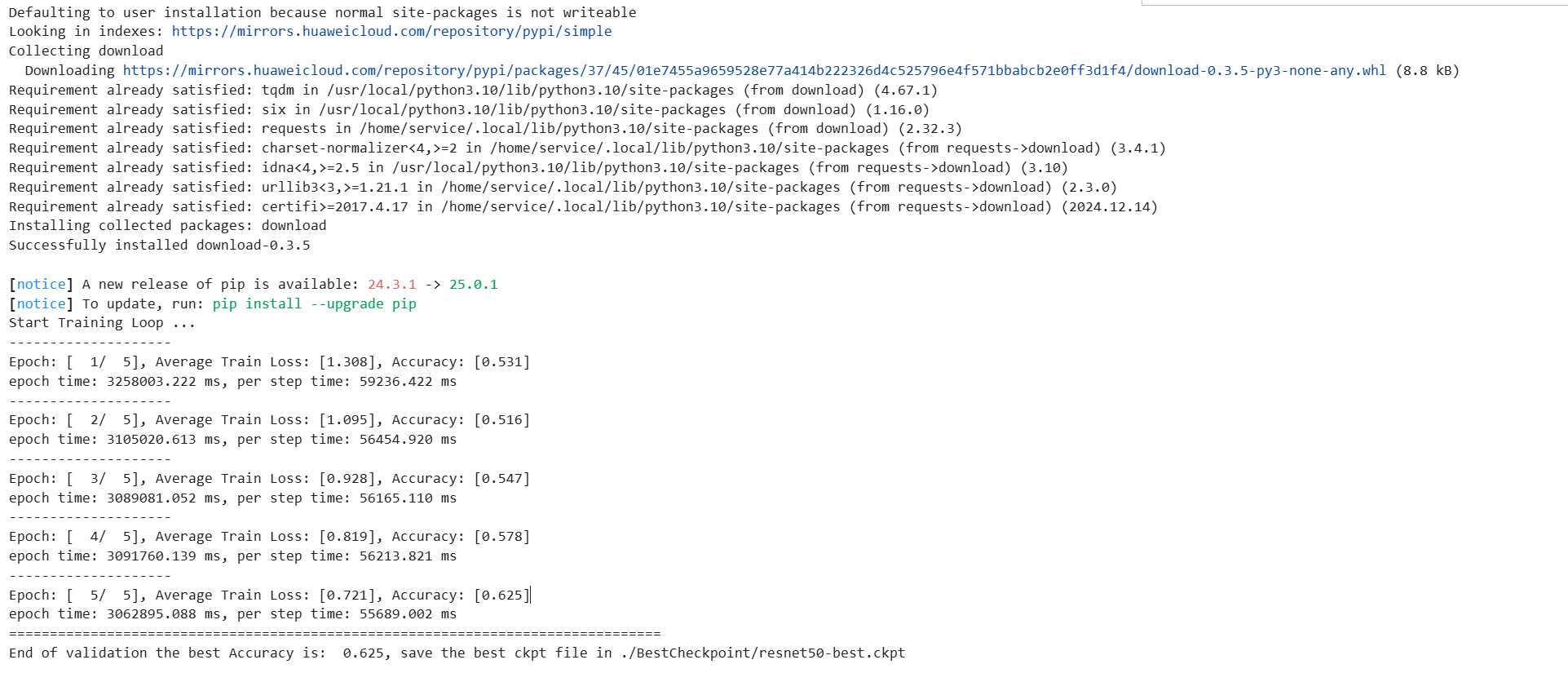
模型训练（训练时长预计40min）

先导入预训练模型文件：新建pretrainmodel文件夹，将以下文件导入：

resnet50_224_new.ckpt

命令如下

!mkdir pretrainmodel

!wget -P pretrainmodel <https://mindspore-website.obs.cn-north-4.myhuaweicloud.com/notebook/models/application/resnet50_224_new.ckpt>

# 代码中首先导入了必要的MindSpore模块和函数，并设置了运行环境。
import mindspore
from mindspore import nn, train
from mindspore.nn import Loss, Accuracy
!pip install download
import mindspore as ms
from download import download
network = resnet50(pretrained=True)
# 通过替换ResNet50的原始全连接层和平均池化层来适配新的任务
# 全连接层输入层的大小
in_channels = network.fc.in_channels
# 输出通道数大小为皮肤肿瘤分类数4
head = nn.Dense(in_channels, 4)
# 重置全连接层
network.fc = head
# 平均池化层kernel size为7
avg_pool = nn.AvgPool2d(kernel_size=7)
# 重置平均池化层
network.avg_pool = avg_pool
import mindspore as ms
import mindspore
# 定义优化器和损失函数
opt = nn.Momentum(params=network.trainable_params(), learning_rate=lr, momentum=momentum)
loss_fn = nn.SoftmaxCrossEntropyWithLogits(sparse=True, reduction='mean')
# 实例化模型
model = train.Model(network, loss_fn, opt, metrics={"Accuracy": Accuracy()})
def forward_fn(inputs, targets):
logits = network(inputs)
loss = loss_fn(logits, targets)
return loss
grad_fn = mindspore.ops.value_and_grad(forward_fn, None, opt.parameters)
def train_step(inputs, targets):
loss, grads = grad_fn(inputs, targets)
opt(grads)
return loss
# 创建迭代器
data_loader_train = dataset_train.create_tuple_iterator(num_epochs=num_epochs)
# 最佳模型保存路径
best_ckpt_dir = "./BestCheckpoint"
best_ckpt_path = "./BestCheckpoint/resnet50-best.ckpt"
import os
import time
# 开始循环训练
print("Start Training Loop ...")
best_acc = 0
# 训练循环中，数据通过迭代器被加载，模型在每个epoch中更新权重，并计算训练损失。
# 在每个epoch结束时，模型在验证集上评估准确率，并保存具有最高准确率的模型检查点。
for epoch in range(num_epochs):
losses = []
network.set_train()
epoch_start = time.time()
# 为每轮训练读入数据
for i, (images, labels) in enumerate(data_loader_train):
labels = labels.astype(ms.int32)
loss = train_step(images, labels)
losses.append(loss)
# 每个epoch结束后，验证准确率
acc = model.eval(dataset_val)['Accuracy']
epoch_end = time.time()
epoch_seconds = (epoch_end - epoch_start) * 1000
step_seconds = epoch_seconds/step_size_train
print("-" * 20)
print("Epoch: [%3d/%3d], Average Train Loss: [%5.3f], Accuracy: [%5.3f]" % (
epoch+1, num_epochs, sum(losses)/len(losses), acc
))
print("epoch time: %5.3f ms, per step time: %5.3f ms" % (
epoch_seconds, step_seconds
))
if acc > best_acc:
best_acc = acc
if not os.path.exists(best_ckpt_dir):
os.mkdir(best_ckpt_dir)
ms.save_checkpoint(network, best_ckpt_path)
print("=" * 80)
print(f"End of validation the best Accuracy is: {best_acc: 5.3f}, "
f"save the best ckpt file in {best_ckpt_path}", flush=True)

注释：定义模型训练的步骤，包括前向传播、反向传播、优化器和损失函数的设置，以及模型的训练和评估过程，保存最佳模型检查点。

分析：训练过程是模型学习数据特征的关键阶段，评估阶段用于监控模型的泛化能力，保存最佳模型可以用于后续的预测和部署。

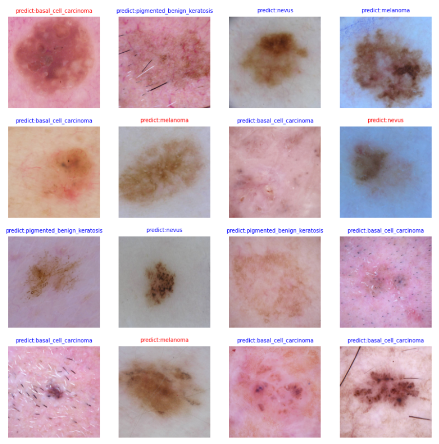
模型评估

import matplotlib.pyplot as plt
import mindspore as ms
def visualize_model(best_ckpt_path, val_ds):
net = resnet50()
# 全连接层输入层的大小
in_channels = net.fc.in_channels
# 输出通道数大小为分类数4
head = nn.Dense(in_channels, 4)
# 重置全连接层
net.fc = head
# 平均池化层kernel size为7
avg_pool = nn.AvgPool2d(kernel_size=7)
# 重置平均池化层
net.avg_pool = avg_pool
# 加载模型参数
param_dict = ms.load_checkpoint(best_ckpt_path)
ms.load_param_into_net(net, param_dict)
model = train.Model(net)
# 加载验证集的数据进行验证
data = next(val_ds.create_dict_iterator())
images = data["image"].asnumpy()
labels = data["label"].asnumpy()
#print(labels)
class_name = {
0: "basal_cell_carcinoma",
1: "melanoma",
2: "nevus",
3: "pigmented_benign_keratosis"
}
# 预测图像类别
data_pre=ms.Tensor(data["image"])
output = model.predict(data_pre)
# print(output)
pred = np.argmax(output.asnumpy(), axis=1)
# 显示图像及图像的预测值
plt.figure(figsize=(10, 10))
for i in range(16):
plt.subplot(4, 4, i + 1)
# 若预测正确，显示为蓝色；若预测错误，显示为红色
color = 'blue' if pred[i] == labels[i] else 'red'
plt.title('predict:{}'.format(class_name[pred[i]]), color=color,fontsize=7)
picture_show = np.transpose(images[i], (1, 2, 0))
mean = np.array([0.485, 0.456, 0.406])
std = np.array([0.229, 0.224, 0.225])
picture_show = std * picture_show + mean
picture_show = np.clip(picture_show, 0, 1)
plt.imshow(picture_show)
plt.axis('off')
plt.show()
visualize_model('BestCheckpoint/resnet50-best.ckpt', dataset_val)

从验证数据集中提取了一批次的数据，使用模型进行预测，并根据预测结果将图像及其预测标签以蓝色（正确）或红色（错误）显示。

使用matplotlib库绘制了一个包含四个子图的图像，每个子图展示了一张图像及其预测结果。

推理使用

import numpy as np
import matplotlib.pyplot as plt
import mindspore as ms
from mindspore import nn
from mindspore.train.serialization import load_checkpoint, load_param_into_net
import mindspore.numpy as mnp
def preprocess_image(image_path):
# 使用PIL加载图像
from PIL import Image
image = Image.open(image_path)
# 转换图像为RGB模式
image = image.convert('RGB')
# 调整图像大小以匹配模型输入
image = image.resize((224, 224)) # 假设模型输入大小为224x224
# 将图像转换为numpy数组
image_array = np.array(image)
# 归一化图像数组
image_array = image_array / 255.0
image_array = np.transpose(image_array, (2, 0, 1))
# 扩展维度以匹配模型输入，例如 (1, 3, 224, 224)
image_array = np.expand_dims(image_array, axis=0)
return image_array.astype(np.float32) # 确保数据类型为float32
def visualize_prediction(image_path, best_ckpt_path):
net = resnet50()
# 全连接层输入层的大小
in_channels = net.fc.in_channels
# 输出通道数大小为分类数4
head = nn.Dense(in_channels, 4)
# 重置全连接层
net.fc = head
# 平均池化层kernel size为7
avg_pool = nn.AvgPool2d(kernel_size=7)
# 重置平均池化层
net.avg_pool = avg_pool
# 加载模型参数
param_dict = ms.load_checkpoint(best_ckpt_path)
ms.load_param_into_net(net, param_dict)
model = train.Model(net)
# 预处理图像
image = preprocess_image(image_path)
data_pre = ms.Tensor(image)
print(data_pre.shape)
print(type(data_pre))
class_name = {
0: "basal_cell_carcinoma",
1: "melanoma",
2: "nevus",
3: "pigmented_benign_keratosis"
}
output = model.predict(data_pre)
print(output)
pred = np.argmax(output.asnumpy(), axis=1)
print(pred)
plt.figure(figsize=(5, 5))
plt.subplot(1, 1, 1)
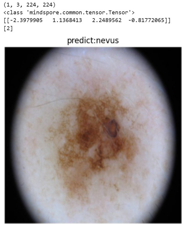
plt.title('predict:{}'.format(class_name[pred[0]]))
picture_show = image[0] # 已经是归一化后的图像
picture_show = np.transpose(picture_show, (1, 2, 0)) # 转换为(224, 224, 3)
plt.imshow(picture_show)
plt.axis('off')
plt.show()
# 调用函数，传入图片路径和模型检查点路径
visualize_prediction('pifudata_Maker/images/val/2/ISIC_0000005.jpg','BestCheckpoint/resnet50-best.ckpt')