【Distributed】分布式监控系统zabbix应用(一)

分布式任务监控体系构建:从设计到落地的全链路实践 在微服务与分布式系统架构中,任务调度与异步处理是支撑业务稳定运行的核心组件。其原理在于通过解耦与并行化提升系统吞吐量与可靠性,但随之而来的便是任务执行过程的可观测性挑战。监控体系的技术价值在于将后台作业从“黑盒”变为“白盒”,实现从任务创建、调度、执行到完成的全生命周期追踪,从而快速定位故障、保障SLA。这通常涉及对任务状态、性能指标、资源消耗及业务自定义数据的采集与分析。在应用场景上,无论是基于Celery、Airflow的定时任务,还是依托Kafka、RabbitMQ的消息队列处理,都需要一套统一的监控 阅读详情

文章目录


前言

  作为一个运维,需要会使用监控系统查看服务器系统性能、应用服务状态和网站流量指标等,利用监控系统的数据去了解网站上线发布的结果和健康状态。

  利用一个优秀的监控软件,我们可以实现以下三种方式:

  1. 通过一个友好的界面进行浏览整个网站所有的服务器状态;
  2. 可以在 Web 前端方便的查看监控数据;
  3. 可以回溯寻找事故发生时系统的问题和报警情况。

一、Zabbix基本概述

1. Zabbix 的概念

  zabbix 是一个基于 Web 界面的提供分布式系统监视以及网络监视功能的企业级的开源解决方案。

  zabbix 能监视各种网络参数,保证服务器系统的安全运营;并提供灵活的通知机制以让系统管理员快速定位/解决存在的各种问题。

2. Zabbix 的工作原理

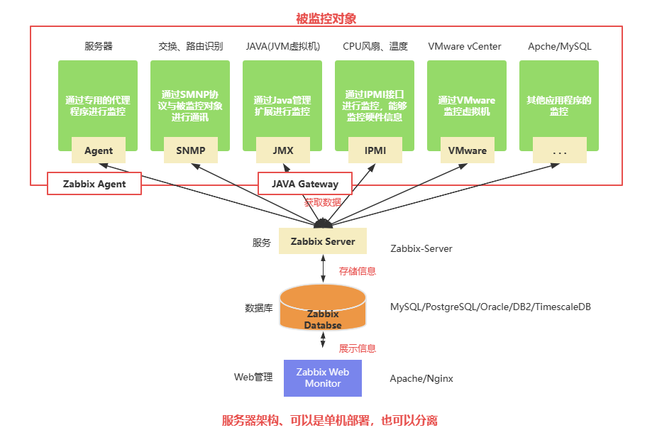
  zabbix agent 安装在被监控的主机上,zabbix agent 负责定期收集客户端本地各项数据,并发送至 zabbix server 端,zabbix server 收到数据后, 将数据存储到数据库中,用户基于 Zabbix Web 可以看到数据在前端展现图像。当 zabbix 监控某个具体的项目, 该项目会设置一个触发器阈值, 当被监控的指标超过该触发器设定的阈值,会进行一些必要的动作,动作包括:发送信息(邮件、微信、短信)、发送命令(shell 命令、reboot、restart、 install 等)。

  总结:zabbix通过采集、存储、处理和展示监控数据,帮助管理员实时监控网络设备和应用程序的运行状态,及时发现和解决问题,提高系统的可用性和稳定性。

3. Zabbix 6.0 新特性

3.1 Zabbix 可以实现高可用

Zabbix server高可用防止硬件故障或计划维护期的停机:

  • 原生选择加入HA群集配置;
  • 定义一个或多个备用节点;
  • 实时监控 Zabbix server 群集节点的状态;
  • 不需要外部工具即可将 Zabbix server配置为HA群集模式。

3.2 Zabbix 新增监控系统

Zabbix 6.0 LTS 新增 Kubernetes 监控功能,可以在 Kubernetes 系统从多个维度采集指标:

  • Kubernetes节点和pods的自动发现和监控;
  • 无代理方式采集 Kubernetes pods和节点的信息;
  • 获取Kubernetes节点主机高水平信息。

4. Zabbix 的构成

  zabbix 由 2 部分构成,zabbix server 与可选组件 zabbix agent。通过 C/S 模式采集数据,通过 B/S 模式在 Web 端展示和配置。

  zabbix server 可以通过 zabbix agent,SNMP协议,端口监视等方法提供对远程服务器/网络状态的监视,数据收集等功能,它可以运行在 Linux 等平台上。

  zabbix agent 需要安装在被监视的目标服务器上,它主要完成对硬件信息或与操作系统有关的内存,CPU 等信息的收集。

5. Zabbix 的功能组件

  Zabbix 服务端(Zabbix Server)守护进程,是 Zabbix 软件的核心组件,Zabbix Agent 向其报告可用性、系统完整性信息和统计信息。Zabbix Server 是存储所有配置信息、统计信息和操作信息的核心存储库。Zabbix Server 也是 Zabbix 监控系统的告警中心。在监控的系统中出现任何异常,将发出通知给管理员。

  基本的 Zabbix Server 的功能分解成为三个不同的组件。他们是:Zabbix server、Web 前端、数据库。

  Zabbix 的所有配置信息都存储在 Server 和 Web 前端进行交互的数据库中。例如,当你通过 Web 前端(或者API)新增一个监控项时, 它会被添加到数据库的监控项表里。然后,Zabbix server 以每分钟一次的频率查询监控项表中的有效项,接着将它存储在 Zabbix server 中的缓存里。 这就是为什么 Zabbix 前端所做的任何更改需要花费两分钟左右才能显示在最新的数据段的原因。

5.1 数据库

  所有配置信息以及 Zabbix 采集到的数据都被持久存储在数据库中。

  可以支持 MySQL、PostgreSQL、Oracle、DB2、TimescaleDB 等多种数据库。

5.2 Web 界面

  Web 界面是 Zabbix Server 的一部分,用于实现展示和配置的界面。通常(但不一定)和 Zabbix server 运行在同一台物理机器上。

  基于 Apache/Nginx + PHP 实现,早期只支持 LAMP 架构,从 Zabbix5.0 开始支持 LNMP 。

5.3 Zabbix Agent

  客户端守护进程,部署在被监控目标上,用于主动监控本地资源和应用程序,并将收集的数据发送给 Zabbix Server。从 Zabbix5.0 开始支技 Zabbix Agent2 。

5.4 Zabbix Proxy

  zabbix 分布式代理守护进程,可以代替 Zabbix Server 采集性能和可用性数据。Zabbix Proxy 在 Zabbix 的部署是可选部分。

  Zabbix Proxy 的部署可以很好的分担单个 Zabbix Server 的负载。

  通常监控大于 500 台主机时使用,需要进行分布式监控架构部署。

5.5 Java Gateway

  Zabbix 要监控 Tomcat 服务或其它 JAVA 程序(比例 Elasticsearch、ZooKeeper),需要使用 Java Gateway 做为代理,才能从 JAVA 程序中获取数据。
在这里插入图片描述

6. Zabbix 和 Prometheus 区别

Zabbix Prometheus
发行时间 2012 2016
开发语言 c+php go
性能 上限约10000节点 支持万为单位
社区支持 应用广泛,支持较成熟,遇到问题都能搜索到 相对不如zabbix,但人数与日俱增
容器支持 Zabbix出现的比较早,当时容器还没有诞生,自然对容器的支持也比较差 不仅支持swarm原生集群,还支持Kubernetes容器集群的监控,是目前容器监控最好解决方案
企业使用 在传统监控系统中,尤其是在服务器相关监控方面,占据绝对优势 基本上使用kubernetes与容器的企业,prometheus是最好的选择
部署难度 多种系统,多种监控信息采集方式 只有一个核心server组件,一条命令便可以启动

二、Zabbix服务器部署

系统:CentOS 7 不支持 yum 方式安装 Zabbix 6.0 服务端

安装方式:Zabbix 服务端采用编译安装的方式,zabbix 客户端采用 yum 安装的方式

1. 部署 Zabbix 服务端

1.1 环境配置

服务器IP地址:192.168.145.30

#关闭 selinux 与防火墙
systemctl disable --now firewalld
setenforce 0
#修改主机名
hostnamectl set-hostname zbx-server

在这里插入图片描述

1.2 部署 Nginx + PHP 环境并测试

#安装 nginx
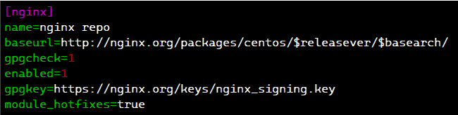
cat > /etc/yum.repos.d/nginx.repo << 'EOF'
[nginx]
name=nginx repo
baseurl=http://nginx.org/packages/centos/$releasever/$basearch/
gpgcheck=1
enabled=1
gpgkey=https://nginx.org/keys/nginx_signing.key
module_hotfixes=true
EOF

yum install -y nginx
[外链图片转存失败,源站可能有防盗链机制,建议将图片保存下来直接上传(img-WGC0LPGa-1688541258972)(C:\Users\86138\AppData\Roaming\Typora\typora-user-images\image-20230705140318479.png)]

#安装 php
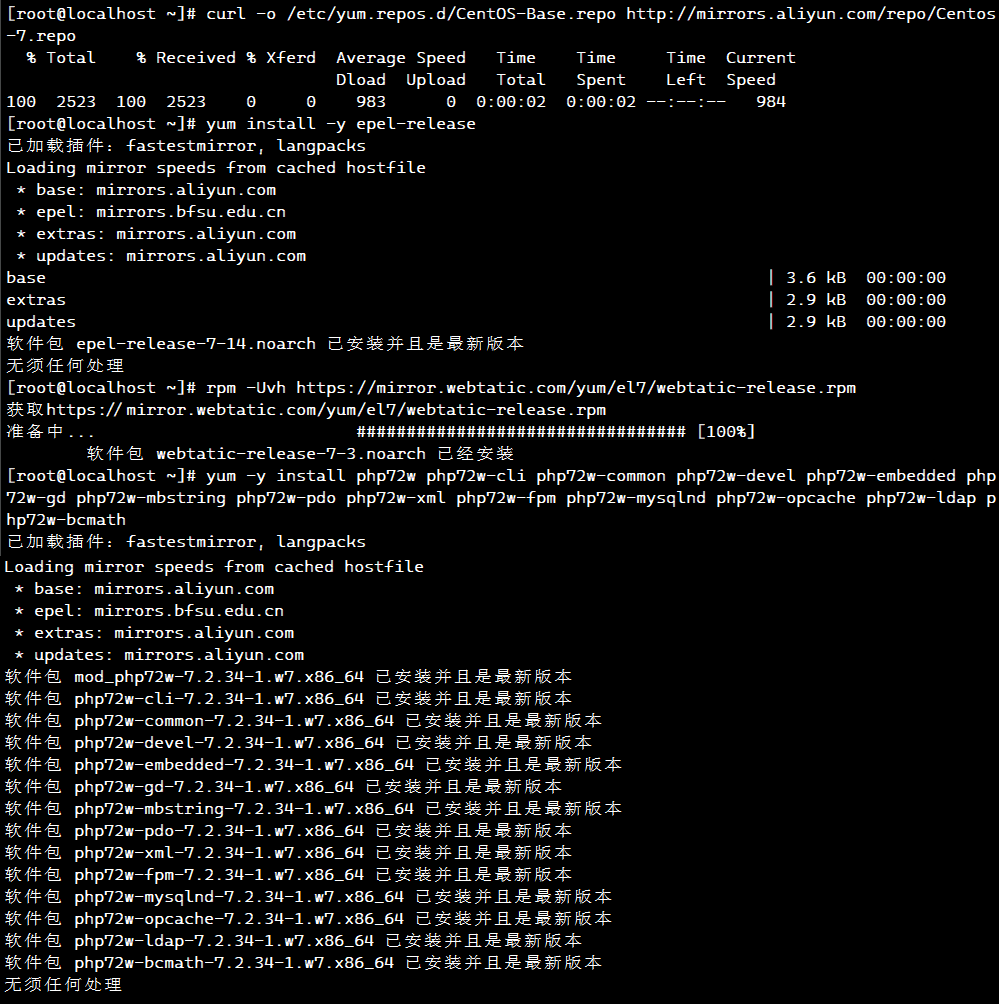
curl -o /etc/yum.repos.d/CentOS-Base.repo http://mirrors.aliyun.com/repo/Centos-7.repo
yum install -y epel-release
rpm -Uvh https://mirror.webtatic.com/yum/el7/webtatic-release.rpm
yum -y install php72w php72w-cli php72w-common php72w-devel php72w-embedded php72w-gd php72w-mbstring php72w-pdo php72w-xml php72w-fpm php72w-mysqlnd php72w-opcache php72w-ldap php72w-bcmath
在这里插入图片描述

#修改 nginx 配置
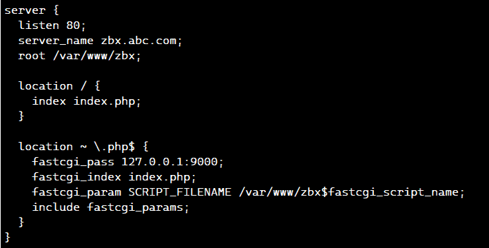
vim /etc/nginx/conf.d/zbx.conf
server {
  listen 80;
  server_name zbx.abc.com;
  root /var/www/zbx;
  
  location / {
    index index.php;
  }
  
  location ~ \.php$ {
    fastcgi_pass 127.0.0.1:9000;
    fastcgi_index index.php;
    fastcgi_param SCRIPT_FILENAME /var/www/zbx$fastcgi_script_name;
    include fastcgi_params;
  }
}
在这里插入图片描述

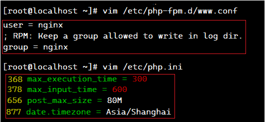
#修改 fpm 配置
vim /etc/php-fpm.d/www.conf
user = nginx
group = nginx

#修改 php 配置
vim /etc/php.ini
max_execution_time = 300		# 368行,最大执行时间
max_input_time = 600			# 378行,超时时间
post_max_size = 80M				# 656行,最大连接数
date.timezone = Asia/Shanghai	# 877行,时区
在这里插入图片描述

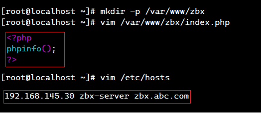
#创建目录和测试文件
mkdir -p /var/www/zbx

vim /var/www/zbx/index.php
<?php
phpinfo();
?>


#配置域名解析
vim /etc/hosts
192.168.145.30 zbx-server zbx.abc.com
在这里插入图片描述

#启动服务
systemctl start nginx php-fpm.service
systemctl enable nginx php-fpm.service

#查看服务状态
netstat -lntp | grep nginx

保姆级教程:vCenter 6.7到8.0.1升级全流程(含LACP配置避坑指南) 本文提供了从vCenter Server 6.7升级至8.0.1的详细全流程指南。重点剖析了升级前的环境评估、关键步骤,并特别针对使用了分布式交换机和LACP配置的网络环境,给出了具体的避坑方案和迁移操作指南,确保升级过程平滑、安全。 阅读详情

相关推荐

VMware ESXi管理IP修改实战:从原理到排错的全流程指南

在虚拟化与服务器运维领域,网络配置是基础且关键的技术环节。其核心原理在于通过IP地址、子网掩码、网关等参数定义设备在网络中的逻辑位置与通信规则。对于VMware ESXi这类专为虚拟化设计的操作系统,其网络架构尤为特殊,管理网络通常绑定在特定的VMkernel端口上,负责主机管理、vCenter通信等核心流量。正确配置管理IP不仅能保障管理通道的稳定,更是实现高效运维、自动化部署以及业务连续性的技术基石。在实际的服务器运维、数据中心迁移或网络架构调整等应用场景中,修改ESXi管理IP是一项常见但需谨慎对待的

weixin_30444111的博客 285

distributed:分布式是基于Next.js的Jamstack应用程序,用于实时社交聊天

分散式 分布式是基于Next.js的Jamstack应用程序,用于实时社交聊天 现场演示 在注册现场演示。 用法 在开始之前,Distributed需要以下环境变量。 # The micro API endpoint MICRO_API_ENDPOINT=https://api.m3o.com # Sendgrid api key for sending invites SENDGRID_API_KEY=xxxxxxxx # Twilio api key/secret/sid for audio/video calls TWILIO_API_KEY=xxxxxxx TWILIO_API_SECRET=xxxxx TWILIO_ACCOUNT_SID=xxxxxx 然后只需执行npm运行构建并开始 # Starts on port 3000 npm run build && npm sta

Distributed_Systems 3rd Edition

2017 ver 3.01 This is the third edition of “Distributed Systems.” In many ways, it is a huge difference compared to the previous editions, the most important one perhaps being that we have fully integrated the “principles” and “paradigms” by including the latter at appropriate places in the chapters that discussed the principles of distributed systems.

Distributed_computing_with_python.zip

Distributed Computing With Python书和代码, 资料中主要介绍了如何利用Python开发、测试以及调试异步、分布式、高并发的程序, 适合想学习python分布式计算的朋友下载学习。

Distributed System

分布式系统概览,关键文档,只要3分,大家一起学习

distributed.sql

rbac权限模型的表结构,包括用户表,角色表  用户角色表,权限表,角色权限表。其中用户角色表和角色权限表是两张关联表。

CS算法实战:用MATLAB从零实现SAR点目标成像(附完整代码)

本文详细介绍了如何使用MATLAB从零实现SAR点目标CS成像算法,涵盖Chirp Scaling(CS)算法的核心理论、距离徙动校正(RCMC)和方位压缩等关键步骤。通过完整的代码示例和实战技巧,帮助读者掌握SAR成像处理算法,提升遥感图像处理能力。

weixin_29211309的博客 179

单细胞拟时序分析实战:用monocle2从Seurat对象构建细胞轨迹(附完整代码)

本文提供了一套完整的单细胞拟时序分析实战教程,详细讲解了如何将Seurat对象转换为Monocle2的CellDataSet,并构建细胞命运轨迹。内容涵盖数据转换、轨迹定义基因选择、降维参数调优、可视化技巧及结果生物学验证,旨在帮助研究者解决实际分析中的常见问题,从静态细胞图谱中挖掘动态发育过程。

weixin_29251337的博客 342

科研人必备!用WisPaper搭建个人文献知识库的完整指南(附Zotero联动技巧)

本文详细介绍了如何利用WisPaper搭建高效的个人文献知识库,包括文件命名标准化、文件夹结构设计、语义搜索技巧及与Zotero的深度联动方法。通过智能标签系统和知识图谱功能,科研人员可以快速定位关键文献,提升研究效率。特别适合需要管理大量学术文献的研究者。

weixin_30823001的博客 267

AMBA-ATB spec

AMBA-ATB spec 1. ATB总线的用途及版本 1.1 ATB总线用途 一般来说,ATB(Advanced Trace Bus)总线用来在ARM的coresight组件之间传递trace数据。如下图所示: 1.2 ATB总线的版本 ATB(Advanced Trace Bus)共有两个版本,其中v1.0作为AMBA3的一部分,于2006年发布的,而v1.1则是2012年随着AMBA4发布的。ATB规范新增了数据(主要针对trace data)不可知的接口,以便在跟踪系统中根据 AMBA 规范跟

weixin_43781229的博客 7346

浏览器Cookie迁移实战:从Chrome导出导入登录态全攻略

Cookie是浏览器保存的会话凭证,服务端通过Set-Cookie将登录态种在本地。迁移Cookie本质上是把服务端认可的会话标识搬到新环境,从而免去重复输入账号密码和二次验证的麻烦。在换电脑、切浏览器或重装系统时,掌握Cookie的导出导入技术能显著提升效率。Chrome与Edge同属Chromium内核,存储结构相似,但字段差异(如Domain、SameSite、Secure)常导致迁移失败。通过浏览器扩展或CDP脚本可实现跨浏览器登录态迁移,适用于内网后台、开发环境等场景。本文从原理到实践,梳理Coo

weixin_42533120的博客 339

用 ABAP RAP + XCO 把 Excel 导入业务对象:从弹窗 Action 到 EML 落库与附件清理的完整实践

摘要:本文介绍了在SAP RAP框架下实现Excel批量导入功能的完整方案。通过XCO库的XLSX模块解析Excel文件,结合RAP的行为定义和Fiori Elements界面集成,构建了一个支持试运行、数据校验和自动合并的业务导入功能。方案采用RAP标准范式,包括Action参数设计、EML事务处理、附件管理以及异常消息反馈,实现了从文件上传到数据落库的端到端流程,既保证了系统稳定性,又提升了业务用户体验。

2007 年 ~ 2025 年,深耕 SAP 技术 18 年 275

SAP ABAP 缓冲同步揭秘——从 DDLOG 表到 RSDBBUF3 的完整实践指南

DDLOG 看似一张不起眼的系统表,却承担着 SAP 多实例环境下的数据一致性重任。通过掌握其字段意义、解析方法及周边监控工具,你可以在性能与一致性之间找到最佳平衡;通过精细化的参数管理与主动刷新策略,更能在关键业务场景中确保“数据永远是最新的”。愿本文能成为你日常排障与架构决策的参考手册。

2007 年 ~ 2025 年,深耕 SAP 技术 18 年 312

【RKNN】RKNN(Rockchip Neural Network)​​ 的详解

RKNN 为 Rockchip 硬件提供了高效的 AI 推理解决方案,适合需要低功耗、实时响应的边缘场景

浩瀚之水的专栏 1684

jre9下载 jdk9

(Java SE Runtime Environment 9.0) 9.0u175 官方最新版 【x86|x64】

visio安装包

Microsoft Office Visio 是一款专业的制图软件。利用经过更新的形状、协作工具和数据链接图表,创建专业级图表以简化复杂的信息。

深度学习工具包 DeepLearningToolbox

深度学习工具包Deprecation notice.-----This toolbox is outdated and no longer maintained.There are much better tools available for deep learning than this toolbox, e.g. [Theano](http://deeplearning.net/software/theano/), [torch](http://torch.ch/) or [tensorflow](http://www.tensorflow.org/)I would suggest you use one of the tools mentioned above rather than use this toolbox.Best, Rasmus.DeepLearnToolbox================A Matlab toolbox for Deep Learning.Deep Learning is a new subfield of machine learning that focuses on learning deep hierarchical models of data.It is inspired by the human brain's apparent deep (layered, hierarchical) architecture.A good overview of the theory of Deep Learning theory is[Learning Deep Architectures for AI](http://www.iro.umontreal.ca/~bengioy/papers/ftml_book.pdf)For a more informal introduction, see the following videos by Geoffrey Hinton and Andrew Ng.* [The Next Generation of Neural Networks](http://www.youtube.com/watch?v=AyzOUbkUf3M) (Hinton, 2007)* [Recent Developments in Deep Learning](http://www.youtube.com/watch?v=VdIURAu1-aU) (Hinton, 2010)* [Unsupervised Feature Learning and Deep Learning](http://www.youtube.com/watch?v=ZmNOAtZIgIk) (Ng, 2011)If you use this toolbox in your research please cite [Prediction as a candidate for learning deep hierarchical models of data](http://www2.imm.dtu.dk/pubdb/views/publication_details.php?id=6284)```@MASTERSTHESIS\{IMM2012-06284, author = "R. B. Palm", title = "Prediction as a candidate for learning deep hierarchical models of data", year = "2012",}```Contact: rasmusbergpalm at gmail dot comDirectories included in the toolbox-----------------------------------`NN/` - A library for Feedforward Backpropagation Neural Networks`CNN/` - A library for Convolutional Neural Networks`DBN/` - A library for Deep Belief Networks`SAE/` - A library for Stacked Auto-Encoders`CAE/` - A library for Convolutional Auto-Encoders`util/` - Utility functions used by the libraries`data/` - Data used by the examples`tests/` - unit tests to verify toolbox is workingFor references on each library check REFS.mdSetup-----1. Download.2. addpath(genpath('DeepLearnToolbox'));Example: Deep Belief Network---------------------```matlabfunction test_example_DBNload mnist_uint8;train_x = double(train_x) / 255;test_x = double(test_x) / 255;train_y = double(train_y);test_y = double(test_y);%% ex1 train a 100 hidden unit RBM and visualize its weightsrand('state',0)dbn.sizes = [100];opts.numepochs = 1;opts.batchsize = 100;opts.momentum = 0;opts.alpha = 1;dbn = dbnsetup(dbn, train_x, opts);dbn = dbntrain(dbn, train_x, opts);figure; visualize(dbn.rbm{1}.W'); % Visualize the RBM weights%% ex2 train a 100-100 hidden unit DBN and use its weights to initialize a NNrand('state',0)%train dbndbn.sizes = [100 100];opts.numepochs = 1;opts.batchsize = 100;opts.momentum = 0;opts.alpha = 1;dbn = dbnsetup(dbn, train_x, opts);dbn = dbntrain(dbn, train_x, opts);%unfold dbn to nnnn = dbnunfoldtonn(dbn, 10);nn.activation_function = 'sigm';%train nnopts.numepochs = 1;opts.batchsize = 100;nn = nntrain(nn, train_x, train_y, opts);[er, bad] = nntest(nn, test_x, test_y);assert(er < 0.10, 'Too big error');```Example: Stacked Auto-Encoders---------------------```matlabfunction test_example_SAEload mnist_uint8;train_x = double(train_x)/255;test_x = double(test_x)/255;train_y = double(train_y);test_y = double(test_y);%% ex1 train a 100 hidden unit SDAE and use it to initialize a FFNN% Setup and train a stacked denoising autoencoder (SDAE)rand('state',0)sae = saesetup([784 100]);sae.ae{1}.activation_function = 'sigm';sae.ae{1}.learningRate = 1;sae.ae{1}.inputZeroMaskedFraction = 0.5;opts.numepochs = 1;opts.batchsize = 100;sae = saetrain(sae, train_x, opts);visualize(sae.ae{1}.W{1}(:,2:end)')% Use the SDAE to initialize a FFNNnn = nnsetup([784 100 10]);nn.activation_function = 'sigm';nn.learningRate = 1;nn.W{1} = sae.ae{1}.W{1};% Train the FFNNopts.numepochs = 1;opts.batchsize = 100;nn = nntrain(nn, train_x, train_y, opts);[er, bad] = nntest(nn, test_x, test_y);assert(er < 0.16, 'Too big error');```Example: Convolutional Neural Nets---------------------```matlabfunction test_example_CNNload mnist_uint8;train_x = double(reshape(train_x',28,28,60000))/255;test_x = double(reshape(test_x',28,28,10000))/255;train_y = double(train_y');test_y = double(test_y');%% ex1 Train a 6c-2s-12c-2s Convolutional neural network %will run 1 epoch in about 200 second and get around 11% error. %With 100 epochs you'll get around 1.2% errorrand('state',0)cnn.layers = { struct('type', 'i') %input layer struct('type', 'c', 'outputmaps', 6, 'kernelsize', 5) %convolution layer struct('type', 's', 'scale', 2) %sub sampling layer struct('type', 'c', 'outputmaps', 12, 'kernelsize', 5) %convolution layer struct('type', 's', 'scale', 2) %subsampling layer};cnn = cnnsetup(cnn, train_x, train_y);opts.alpha = 1;opts.batchsize = 50;opts.numepochs = 1;cnn = cnntrain(cnn, train_x, train_y, opts);[er, bad] = cnntest(cnn, test_x, test_y);%plot mean squared errorfigure; plot(cnn.rL);assert(er<0.12, 'Too big error');```Example: Neural Networks---------------------```matlabfunction test_example_NNload mnist_uint8;train_x = double(train_x) / 255;test_x = double(test_x) / 255;train_y = double(train_y);test_y = double(test_y);% normalize[train_x, mu, sigma] = zscore(train_x);test_x = normalize(test_x, mu, sigma);%% ex1 vanilla neural netrand('state',0)nn = nnsetup([784 100 10]);opts.numepochs = 1; % Number of full sweeps through dataopts.batchsize = 100; % Take a mean gradient step over this many samples[nn, L] = nntrain(nn, train_x, train_y, opts);[er, bad] = nntest(nn, test_x, test_y);assert(er < 0.08, 'Too big error');%% ex2 neural net with L2 weight decayrand('state',0)nn = nnsetup([784 100 10]);nn.weightPenaltyL2 = 1e-4; % L2 weight decayopts.numepochs = 1; % Number of full sweeps through dataopts.batchsize = 100; % Take a mean gradient step over this many samplesnn = nntrain(nn, train_x, train_y, opts);[er, bad] = nntest(nn, test_x, test_y);assert(er < 0.1, 'Too big error');%% ex3 neural net with dropoutrand('state',0)nn = nnsetup([784 100 10]);nn.dropoutFraction = 0.5; % Dropout fraction opts.numepochs = 1; % Number of full sweeps through dataopts.batchsize = 100; % Take a mean gradient step over this many samplesnn = nntrain(nn, train_x, train_y, opts);[er, bad] = nntest(nn, test_x, test_y);assert(er < 0.1, 'Too big error');%% ex4 neural net with sigmoid activation functionrand('state',0)nn = nnsetup([784 100 10]);nn.activation_function = 'sigm'; % Sigmoid activation functionnn.learningRate = 1; % Sigm require a lower learning rateopts.numepochs = 1; % Number of full sweeps through dataopts.batchsize = 100; % Take a mean gradient step over this many samplesnn = nntrain(nn, train_x, train_y, opts);[er, bad] = nntest(nn, test_x, test_y);assert(er < 0.1, 'Too big error');%% ex5 plotting functionalityrand('state',0)nn = nnsetup([784 20 10]);opts.numepochs = 5; % Number of full sweeps through datann.output = 'softmax'; % use softmax outputopts.batchsize = 1000; % Take a mean gradient step over this many samplesopts.plot = 1; % enable plottingnn = nntrain(nn, train_x, train_y, opts);[er, bad] = nntest(nn, test_x, test_y);assert(er < 0.1, 'Too big error');%% ex6 neural net with sigmoid activation and plotting of validation and training error% split training data into training and validation datavx = train_x(1:10000,:);tx = train_x(10001:end,:);vy = train_y(1:10000,:);ty = train_y(10001:end,:);rand('state',0)nn = nnsetup([784 20 10]); nn.output = 'softmax'; % use softmax outputopts.numepochs = 5; % Number of full sweeps through dataopts.batchsize = 1000; % Take a mean gradient step over this many samplesopts.plot = 1; % enable plottingnn = nntrain(nn, tx, ty, opts, vx, vy); % nntrain takes validation set as last two arguments (optionally)[er, bad] = nntest(nn, test_x, test_y);assert(er < 0.1, 'Too big error');```[![Bitdeli Badge](https://d2weczhvl823v0.cloudfront.net/rasmusbergpalm/deeplearntoolbox/trend.png)](https://bitdeli.com/free "Bitdeli Badge")

迈瑞BS系列全自动生化分析仪LIS协议接口手册(内含HL7和ASTM)

迈瑞BS系列全自动生化分析仪LIS协议接口手册,内含HL7和ASTM)

上一篇: 【Cache】Rsync远程同步
下一篇: 【Distributed】分布式监控系统zabbix应用(二)
我的宝贝大唐
博客等级 码龄7年 96粉丝 111原创
评论
成就一亿技术人!
拼手气红包6.0元
还能输入1000个字符
 
 条评论被折叠 查看
添加红包

请填写红包祝福语或标题

个

红包个数最小为10个

元

红包金额最低5元

当前余额3.43元 前往充值 >
需支付:10.00元
成就一亿技术人!
领取后你会自动成为博主和红包主的粉丝 规则
hope_wisdom
发出的红包

打赏作者

我的宝贝大唐

你的鼓励将是我创作的最大动力

¥1 ¥2 ¥4 ¥6 ¥10 ¥20
扫码支付:¥1
获取中
扫码支付

您的余额不足,请更换扫码支付或充值

打赏作者

实付元
使用余额支付
点击重新获取
扫码支付
钱包余额 0

抵扣说明:

1.余额是钱包充值的虚拟货币,按照1:1的比例进行支付金额的抵扣。
2.余额无法直接购买下载,可以购买VIP、付费专栏及课程。

余额充值