Kaggle: 泰坦尼克号生存预测

0.前言

本文对Kaggle泰坦尼克比赛的训练集和测试集进行分析,并对乘客的生存结果进行了预测.作为数据挖掘的入门项目,本人将思路记录下来,以供参考.如有不足之处,欢迎指正.

1.导入数据

import pandas as pd
import numpy as np
import matplotlib.pyplot as plt
import seaborn as sns

# 忽略警告
import warnings
warnings.filterwarnings('ignore')

train = pd.read_csv('train.csv')
test = pd.read_csv('test.csv')
test_initial = test  #备份测试数据
train_len = len(train)

'''每个特征的含义： 
PassengerId (乘客编号) 
Survived (存活与否) 
Pclass (客舱等级) 
Name (姓名) 
Sex (性别) 
Age (年龄) 
SibSp (兄妹人数) 
Parch (父母子女人数) 
Ticket (船票编号) 
Fare (票价) 
Cabin (客舱位置) 
Embarked (登船地点)
'''

# 查看训练集
train.head(10)

	PassengerId	Survived	Pclass	Name	Sex	Age	SibSp	Parch	Ticket	Fare	Cabin	Embarked
0	1	0	3	Braund, Mr. Owen Harris	male	22.0	1	0	A/5 21171	7.2500	NaN	S
1	2	1	1	Cumings, Mrs. John Bradley (Florence Briggs Th…	female	38.0	1	0	PC 17599	71.2833	C85	C
2	3	1	3	Heikkinen, Miss. Laina	female	26.0	0	0	STON/O2. 3101282	7.9250	NaN	S
3	4	1	1	Futrelle, Mrs. Jacques Heath (Lily May Peel)	female	35.0	1	0	113803	53.1000	C123	S
4	5	0	3	Allen, Mr. William Henry	male	35.0	0	0	373450	8.0500	NaN	S
5	6	0	3	Moran, Mr. James	male	NaN	0	0	330877	8.4583	NaN	Q
6	7	0	1	McCarthy, Mr. Timothy J	male	54.0	0	0	17463	51.8625	E46	S
7	8	0	3	Palsson, Master. Gosta Leonard	male	2.0	3	1	349909	21.0750	NaN	S
8	9	1	3	Johnson, Mrs. Oscar W (Elisabeth Vilhelmina Berg)	female	27.0	0	2	347742	11.1333	NaN	S
9	10	1	2	Nasser, Mrs. Nicholas (Adele Achem)	female	14.0	1	0	237736	30.0708	NaN	C

# 测试集数据缺少Survived这一列,正是我们要预测的列
test.head(10)

	PassengerId	Pclass	Name	Sex	Age	SibSp	Parch	Ticket	Fare	Cabin	Embarked
0	892	3	Kelly, Mr. James	male	34.5	0	0	330911	7.8292	NaN	Q
1	893	3	Wilkes, Mrs. James (Ellen Needs)	female	47.0	1	0	363272	7.0000	NaN	S
2	894	2	Myles, Mr. Thomas Francis	male	62.0	0	0	240276	9.6875	NaN	Q
3	895	3	Wirz, Mr. Albert	male	27.0	0	0	315154	8.6625	NaN	S
4	896	3	Hirvonen, Mrs. Alexander (Helga E Lindqvist)	female	22.0	1	1	3101298	12.2875	NaN	S
5	897	3	Svensson, Mr. Johan Cervin	male	14.0	0	0	7538	9.2250	NaN	S
6	898	3	Connolly, Miss. Kate	female	30.0	0	0	330972	7.6292	NaN	Q
7	899	2	Caldwell, Mr. Albert Francis	male	26.0	1	1	248738	29.0000	NaN	S
8	900	3	Abrahim, Mrs. Joseph (Sophie Halaut Easu)	female	18.0	0	0	2657	7.2292	NaN	C
9	901	3	Davies, Mr. John Samuel	male	21.0	2	0	A/4 48871	24.1500	NaN	S

#查看训练集和测试集的缺失数据, 缺失值较少的是Fare和Embarked, 缺失值较多的是Age和Cabin
train.isnull().sum()

test.isnull().sum()

2.特征分析

2.1 数值数据

# 数值数据: Survived, Age, Sibsp, Parch, Fare, 画热力图查看它们与生存的关系
sns.heatmap(train[["Survived","Age","SibSp","Parch","Fare"]].corr(),annot=True, fmt = ".2f",cmap = "coolwarm")
plt.title('Pearson Correlation of Numerical Features')
plt.show()

# 我们需进一步查看这些特征和生存的关系
# 年龄和生存关系, 小孩的的生存率明显高些
g = sns.FacetGrid(train, hue="Survived",aspect=4)
g.map(sns.kdeplot,'Age',shade= True)
g.set(xlim=(0, train['Age'].max()))
g.add_legend()
plt.show()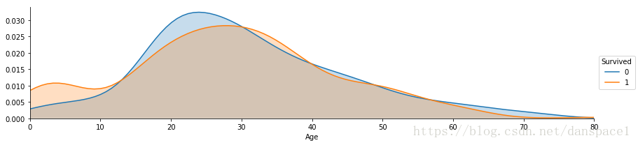

# 兄妹配偶数目与生存的关系,数目为1-2的生存率明显要高
g = sns.factorplot(x="SibSp",y="Survived",data=train,kind="bar")
g.set_ylabels("survival probability")
plt.show()

# 父母子女与生存的关系, 有家人的生存率高于独自一人,家人太多生存率也会下降
g = sns.factorplot(x="Parch",y="Survived",data=train,kind="bar")
g.set_ylabels("survival probability")
plt.show()

# 票价与生存的关系,大多数集中在100以内
g = sns.distplot(train['Fare'],label='skewness:{:.2f}'.format(train['Fare'].skew()))
g.legend(loc="best")
plt.show()

2.2 分类数据

# 性别,女性生存率明显高于男性
g = sns.barplot(x="Sex",y="Survived",data=train)
g.set_ylabel("Survival Probability")
plt.show()

# 客舱等级, 等级越高,生存几率越大
g = sns.barplot(x="Pclass",y="Survived",data=train)
g.set_ylabel("Survival Probability")
plt.show()

# 登船地点, 在C点登船的生存率最高
sns.factorplot(data=train, x="Embarked", y="Survived")
plt.show()

# 客舱位置,由于缺失值很多,将Cabin缺失与否作为条件,看与生存的关系
# 有客舱的生存率明显高于没客舱的
train['Cabin_Bool'] = (train["Cabin"].notnull().astype('int'))
sns.barplot(x="Cabin_Bool", y="Survived", data=train)
plt.show()

3.填充缺失数据

# 合并训练集和测试集
combined = pd.concat([train, test], axis = 0, ignore_index= True)
# 查看缺失数据
combined.isnull().sum()

3.1 填充Fare, Embarked

# Fare, Embarked缺失值很少
# Embarked有2个缺失值,用众数填补
combined.Embarked.value_counts()
combined['Embarked'] = combined['Embarked'].fillna('S')

# Fare缺失值按对应客舱等级的均价来填充, 对应的Pclass为3
combined[combined.Fare.isnull()]

	Age	Cabin	Cabin_Bool	Embarked	Fare	Name	Parch	PassengerId	Pclass	Sex	SibSp	Survived	Ticket
1043	60.5	NaN	NaN	S	NaN	Storey, Mr. Thomas	0	1044	3	male	0	NaN	3701

combined[combined.Pclass==3]['Fare'].mean()

13.302888700564969

combined['Fare'].fillna(value = combined[combined.Pclass==3]['Fare'].mean(), inplace = True)

3.2 填充Age

# Age缺失值有263个,先使用最相关的特征来查看相关性(Sex, Pclass, Parch, SibSp)
fig = plt.figure(figsize=(10,10))
ax1 = fig.add_subplot(221)
ax2 = fig.add_subplot(222)
ax3 = fig.add_subplot(223)
ax4 = fig.add_subplot(224)

sns.boxplot(y='Age',x= 'Sex',data = combined,ax = ax1)
sns.boxplot(y='Age',x= 'Pclass',data = combined,ax = ax2)
sns.boxplot(y='Age',x= 'Parch',data = combined,ax = ax3)
sns.boxplot(y='Age',x= 'SibSp',data = combined,ax = ax4)
plt.show()

# 将Sex转化为数字
combined["Sex"] = combined["Sex"].map({"male": 0, "female":1})

# 查看age和几个特征的相关性, 可见年龄与性别不相关
sns.heatmap(combined[["Age","Sex","SibSp","Parch","Pclass"]].corr(),annot=True, fmt = ".2f",cmap = "coolwarm")
plt.show()

# 根据相似列Pclass, Parch,SibSp的中位数来填充年龄的空值

index_nan_age = list(combined['Age'][combined.Age.isnull()].index)

for i in index_nan_age:
    # 如果相似列不存在,使用整列的中位数
    median_pred = combined['Age'][((combined['SibSp'] == combined.iloc[i]["SibSp"]) & (combined['Parch'] == combined.iloc[i]["Parch"]) & (combined['Pclass'] == combined.iloc[i]["Pclass"]))].median()
    median_col = combined['Age'].median()
    if not np.isnan(median_pred):
        combined['Age'][i] = median_pred
    else:
        combined['Age'][i] = median_col

# 查看数据集
combined.head()

	Age	Cabin	Cabin_Bool	Embarked	Fare	Name	Parch	PassengerId	Pclass	Sex	SibSp	Survived	Ticket
0	22.0	NaN	0.0	S	7.2500	Braund, Mr. Owen Harris	0	1	3	0	1	0.0	A/5 21171
1	38.0	C85	1.0	C	71.2833	Cumings, Mrs. John Bradley (Florence Briggs Th…	0	2	1	1	1	1.0	PC 17599
2	26.0	NaN	0.0	S	7.9250	Heikkinen, Miss. Laina	0	3	3	1	0	1.0	STON/O2. 3101282
3	35.0	C123	1.0	S	53.1000	Futrelle, Mrs. Jacques Heath (Lily May Peel)	0	4	1	1	1	1.0	113803
4	35.0	NaN	0.0	S	8.0500	Allen, Mr. William Henry	0	5	3	0	0	0.0	373450

4.特征工程

4.1 从Name中提取头衔

# Name, 从名称中提取头衔
title = [i.split(',')[1].split('.')[0].strip() for i in combined['Name']]
combined['Title'] = pd.Series(title)
# 查看头衔的分布
plt.figure(figsize=(10,6))
sns.countplot(x="Title",data=combined)
plt.xticks(rotation='45')
plt.show()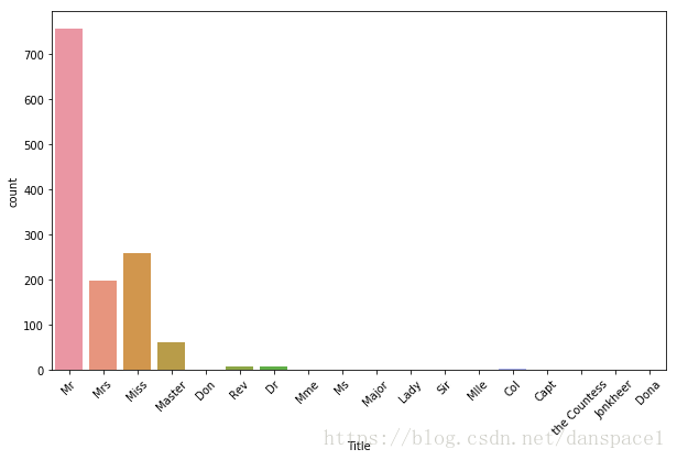

# 将头衔分为4类: Mr,Miss, Master, Rare
combined["Title"].replace(['Don','Rev','Dr','Major','Lady','Sir','Col','Capt','the Countess','Jonkheer', 'Dona'], value='Rare', inplace = True)
combined["Title"] = combined["Title"].map({"Master":0, "Miss":1, "Ms" : 1 , "Mme":1, "Mlle":1, "Mrs":1, "Mr":2, "Rare":3})
combined["Title"].value_counts()

# 头衔与生存的关系
g = sns.barplot(x="Title",y="Survived",data= combined)
g.set(xticklabels = ["Master","Miss-Mrs","Mr","Rare"], ylabel='survival probability')
plt.show()

4.2 从Parch和SibSp中提取家庭人数

# 家庭人数,小家庭的生存率远高于独自一人和大家庭
combined['Fam_Size'] = combined['Parch'] + combined['SibSp'] + 1
sns.factorplot(x="Fam_Size",y="Survived",data = combined)
plt.show()

# 将家人数量归类
def make_category(size):
    if size == 1:
        return 'single'
    elif size <= 3:
        return 'small'
    elif size == 4:
        return 'medium'
    else:
        return 'large'

combined['Fam_Size_Class'] = combined['Fam_Size'].map(make_category)

# 转化为虚拟变量
dummy_fam_size = pd.get_dummies(combined['Fam_Size_Class'],prefix ='Fam_Size')
combined = pd.concat([combined, dummy_fam_size], axis = 1)
combined.head()

	Age	Cabin	Cabin_Bool	Embarked	Fare	Name	Parch	PassengerId	Pclass	Sex	SibSp	Survived	Ticket	Title	Fam_Size	Fam_Size_Class	Fam_Size_large	Fam_Size_medium	Fam_Size_single	Fam_Size_small
0	22.0	NaN	0.0	S	7.2500	Braund, Mr. Owen Harris	0	1	3	0	1	0.0	A/5 21171	2	2	small	0	0	0	1
1	38.0	C85	1.0	C	71.2833	Cumings, Mrs. John Bradley (Florence Briggs Th…	0	2	1	1	1	1.0	PC 17599	1	2	small	0	0	0	1
2	26.0	NaN	0.0	S	7.9250	Heikkinen, Miss. Laina	0	3	3	1	0	1.0	STON/O2. 3101282	1	1	single	0	0	1	0
3	35.0	C123	1.0	S	53.1000	Futrelle, Mrs. Jacques Heath (Lily May Peel)	0	4	1	1	1	1.0	113803	1	2	small	0	0	0	1
4	35.0	NaN	0.0	S	8.0500	Allen, Mr. William Henry	0	5	3	0	0	0.0	373450	2	1	single	0	0	1	0

4.3 从Cabin提取首字母

# 客舱位置, 提取首字母作为乘客在轮船的位置
letter = [i[0] if pd.notnull(i) else 'X' for i in combined['Cabin'] ]
combined['Cabin'] = pd.Series(letter)

fig = plt.figure(figsize=(10,5))
ax1 = fig.add_subplot(121)
ax2 = fig.add_subplot(122)
sns.countplot(combined['Cabin'],order=['A','B','C','D','E','F','G','T','X'], ax=ax1)
sns.barplot(x = combined['Cabin'], y = combined['Survived'], order=['A','B','C','D','E','F','G','T','X'], ax=ax2)
plt.show()

# 将Cabin转化为虚拟变量
combined = pd.get_dummies(combined, columns = ["Cabin"],prefix="Cabin")

4.4 从Ticket中提取字母

# ticket提取字母前缀,如果没有则分类为X, 代表乘客在船上的实际位置,可能与逃生位置有关
Ticket = []
for i in list(combined['Ticket']):
    if not i.isdigit() :
        Ticket.append(i.replace(".","").replace("/","").strip().split(' ')[0]) 
    else:
        Ticket.append("X")

combined["Ticket"] = Ticket
# ticket转化为虚拟变量
combined = pd.get_dummies(combined, columns = ["Ticket"], prefix="Ticket")

combined.head()

	Age	Cabin_Bool	Embarked	Fare	Name	Parch	PassengerId	Pclass	Sex	SibSp	…	Ticket_SOTONO2	Ticket_SOTONOQ	Ticket_SP	Ticket_STONO	Ticket_STONO2	Ticket_STONOQ	Ticket_SWPP	Ticket_WC	Ticket_WEP	Ticket_X
0	22.0	0.0	S	7.2500	Braund, Mr. Owen Harris	0	1	3	0	1	…	0	0	0	0	0	0	0	0	0	0
1	38.0	1.0	C	71.2833	Cumings, Mrs. John Bradley (Florence Briggs Th…	0	2	1	1	1	…	0	0	0	0	0	0	0	0	0	0
2	26.0	0.0	S	7.9250	Heikkinen, Miss. Laina	0	3	3	1	0	…	0	0	0	0	1	0	0	0	0	0
3	35.0	1.0	S	53.1000	Futrelle, Mrs. Jacques Heath (Lily May Peel)	0	4	1	1	1	…	0	0	0	0	0	0	0	0	0	1
4	35.0	0.0	S	8.0500	Allen, Mr. William Henry	0	5	3	0	0	…	0	0	0	0	0	0	0	0	0	1

5 rows × 64 columns

combined.info()

# 将Pclass和Emarked加到虚拟变量
combined = pd.get_dummies(combined, columns = ["Pclass"],prefix="Pclass")
combined = pd.get_dummies(combined, columns = ["Embarked"],prefix="Embarked")
# 剔除不需要的列
combined.drop(['Cabin_Bool','Name','PassengerId','Fam_Size_Class'], axis = 1, inplace = True)
combined.head()

	Age	Fare	Parch	Sex	SibSp	Survived	Title	Fam_Size	Fam_Size_large	Fam_Size_medium	…	Ticket_SWPP	Ticket_WC	Ticket_WEP	Ticket_X	Pclass_1	Pclass_2	Pclass_3	Embarked_C	Embarked_Q	Embarked_S
0	22.0	7.2500	0	0	1	0.0	2	2	0	0	…	0	0	0	0	0	0	1	0	0	1
1	38.0	71.2833	0	1	1	1.0	1	2	0	0	…	0	0	0	0	1	0	0	1	0	0
2	26.0	7.9250	0	1	0	1.0	1	1	0	0	…	0	0	0	0	0	0	1	0	0	1
3	35.0	53.1000	0	1	1	1.0	1	2	0	0	…	0	0	0	1	1	0	0	0	0	1
4	35.0	8.0500	0	0	0	0.0	2	1	0	0	…	0	0	0	1	0	0	1	0	0	1

5 rows × 64 columns

在建模前查看数据集的类别,确保都是数值,才能放进模型里.

combined.info()

5.建模

# 将测试集和训练集分开
train = combined[:train_len]
test = combined[train_len:]

train['Survived'] = train['Survived'].astype(int)
train_Y = train["Survived"]
train_X = train.drop(labels = ["Survived"],axis = 1)
test_X = test.drop(labels=["Survived"],axis = 1)

5.1 交叉验证

# 初步选择6个算法,使用交叉验证检查算法的准确度
# Random Forrest, KNN, Logistic Regression, GradientBoosting,ExtraTrees, AdaBoosting

from sklearn.cross_validation import cross_val_score
from sklearn.ensemble import RandomForestClassifier, VotingClassifier,GradientBoostingClassifier,ExtraTreesClassifier,AdaBoostClassifier
from sklearn.neighbors import KNeighborsClassifier
from sklearn.linear_model import LogisticRegression
from sklearn.tree import DecisionTreeClassifier
from sklearn.model_selection import GridSearchCV, KFold

# Random Forrest
rf_score = cross_val_score(RandomForestClassifier(random_state = 2), X = train_X, y= train_Y, scoring = 'accuracy', cv = 10, n_jobs = -1)
print('Random Forrest: {:.3f}'.format(rf_score.mean()))

# KNN
knn_score = cross_val_score(KNeighborsClassifier(), X = train_X, y= train_Y, scoring = 'accuracy', cv = 10, n_jobs = -1)
print('KNN: {:.3f}'.format(knn_score.mean()))

# Logistic Regression
lr_score = cross_val_score(LogisticRegression(random_state = 2), X = train_X, y= train_Y, scoring = 'accuracy', cv = 10, n_jobs = -1)
print('logistic regresssion: {:.3f}'.format(lr_score.mean()))

# GradientBoosting
gb_score = cross_val_score(GradientBoostingClassifier(random_state = 2), X = train_X, y= train_Y, scoring = 'accuracy', cv = 10, n_jobs = -1)
print('GradientBoosting: {:.3f}'.format(gb_score.mean()))

# ExtraTrees
et_score = cross_val_score(ExtraTreesClassifier(random_state = 2), X = train_X, y= train_Y, scoring = 'accuracy', cv = 10, n_jobs = -1)
print('Extra Tree: {:.3f}'.format(et_score.mean()))

# AdaBoost
ada_score = cross_val_score(AdaBoostClassifier(DecisionTreeClassifier(random_state = 2),random_state = 2, learning_rate = 0.1), X = train_X, y= train_Y, scoring = 'accuracy', cv = 10, n_jobs = -1)
print('Ada Boost: {:.3f}'.format(ada_score.mean()))

Random Forrest: 0.813
KNN: 0.723
logistic regresssion: 0.824
Gradient Boosting: 0.829
Extra Tree: 0.807
Ada Boost: 0.813

5.2 调参

# 交叉验证选出准确率高的模型,选择使用Random Forrest,Logistic Regression,Gradient boosting这3种分类方法.
# 超参数验证:网格搜索,选择能让模型拟合程度最好的参数
kfold = KFold(n_splits=10)

# Random Forrest
rf = RandomForestClassifier()
rf_param_grid = {"max_depth": [None],
              "max_features": [1, 3, 10],
              "min_samples_split": [2, 3, 10],
              "min_samples_leaf": [1, 3, 10],
              "bootstrap": [False],
              "n_estimators" :[100,300],
              "criterion": ["gini"]}

gs_rf = GridSearchCV(rf,param_grid = rf_param_grid, cv=kfold, scoring="accuracy", n_jobs=-1, verbose = 1)

gs_rf.fit(train_X,train_Y)

rf_best = gs_rf.best_estimator_

# Logistic Regression
lr = LogisticRegression()
lr_param_grid = {'C': [0.001, 0.01, 0.1, 1, 10, 100, 1000] }

gs_lr = GridSearchCV(lr,param_grid = lr_param_grid, cv=kfold, scoring="accuracy", n_jobs=-1, verbose = 1)
gs_lr.fit(train_X,train_Y)
lr_best = gs_lr.best_estimator_

# Gradient boosting 
gb = GradientBoostingClassifier()
gb_param_grid = {'loss' : ["deviance"],
              'n_estimators' : [100,200,300],
              'learning_rate': [0.1, 0.05, 0.01],
              'max_depth': [4, 8],
              'min_samples_leaf': [100,150],
              'max_features': [0.3, 0.1] 
              }

gs_gb = GridSearchCV(gb,param_grid = gb_param_grid, cv=kfold, scoring="accuracy", n_jobs= -1, verbose = 1)

gs_gb.fit(train_X,train_Y)

gb_best = gs_gb.best_estimator_

5.3 模型融合

使用投票分类法,将3种模型融合

voting_est = VotingClassifier(estimators = [('rf',rf_best),('lr',lr_best),('gb',gb_best)], voting = 'soft', n_jobs = -1)
voting_est.fit(train_X, train_Y)
predictions = voting_est.predict(test_X)

5.4 生成预测结果

result = pd.DataFrame({'PassengerId': test_initial['PassengerId'], 'Survived': predictions})
result.to_csv('result.csv', index = False)

提交结果,分数如下. 第一次参赛,结果不算差, 但还有改进的空间, 要继续努力呀.