使用Excel INDEX和MATCH检查多个条件

Use INDEX and MATCH together, for a powerful lookup formula. It's similar to a VLOOKUP formula, but more flexible -- the item that you're looking for doesn't have to be in the first column at the left. Watch the video to see how it works (there are written instructions too), and download the sample workbook to follow along.

结合使用INDEX和MATCH，可获得强大的查找公式。 它类似于VLOOKUP公式，但更灵活-您要查找的项目不必在左侧的第一列中。 观看视频以了解其工作原理(也有书面说明)，然后下载示例工作簿进行后续操作。

具有两个条件的Excel查找 (Excel Lookup With Two Criteria)

Watch this video to see how INDEX and MATCH work together -- first with one criterion, and then with multiple criteria. Download the sample workbook to follow along, and the written instructions are below the video.

观看此视频以了解INDEX和MATCH如何一起工作-首先使用一个条件，然后使用多个条件。 下载示例工作簿以进行后续操作，书面说明在视频下方。

演示地址

• 0:00 Introduction
  0:00简介
• 0:26 Lookup with One Criterion
  0:26一种标准的查找
• 1:52 Test Each Criterion
  1:52测试每个标准
• 2:22 Test With a Formula
  2:22用公式测试
• 3:26 Multiply the Results
  3:26将结果相乘
• 4:03 INDEX / MATCH Formula
  4:03 INDEX / MATCH公式
• 5:20 Check the Formula
  5:20检查公式
• 5:57 Get the Sample File
  5:57获取样本文件

使用INDEX和MATCH获取商品价格 (Get Item Price with INDEX and MATCH)

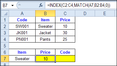
To see how INDEX and MATCH work together, we'll start with an example that has only 1 criterion. Our price list has item names in column B, and we want to get the matching price from column C.

为了了解INDEX和MATCH如何一起工作，我们将从一个只有1个条件的示例开始。 我们的价格表在B列中有商品名称，我们希望从C列中获得匹配的价格。

In the screen shot below, cell A7 has the name of the item that we need a price for - Sweater.

在下面的屏幕快照中，单元格A7中有一个我们需要价格的商品名称-毛衣。

We can enter an INDEX and MATCH formula in cell C7, to get the price for that item:

我们可以在单元格C7中输入INDEX和MATCH公式，以获取该商品的价格：

=INDEX($C$2:$C$4,MATCH(A7,$B$2:$B$4,0))

= INDEX($ C $ 2：$ C $ 4，MATCH(A7，$ B $ 2：$ B $ 4,0))

INDEX和MATCH公式的工作原理 (How the INDEX and MATCH Formula Works)

Here's how the two functions work together:

这两个功能如何一起工作：

•  MATCH function gets the location of an item in a list

  MATCH函数获取项目在列表中的位置

• INDEX function returns a value from a specific location in a list.

  INDEX函数从列表中的特定位置返回一个值。

So, in our formula:

因此，在我们的公式中：

• the MATCH function looks for "Sweater" in the range B2:B4.
  MATCH函数在B2：B4范围内查找“毛衣”。
• The result is 1, because "Sweater" is item number 1, in that range of cells.
  结果为1，因为在该单元格范围内，“毛衣”的编号为1。
• the INDEX function looks in the range C2:C4
  INDEX函数的范围为C2：C4
• The result is 10, from row 1 in that range
  结果是该范围内第1行的10

So, by combining INDEX and MATCH, you can find the row with "Sweater" and return the price from that row.

因此，通过结合INDEX和MATCH，您可以找到带有“毛衣”的行，并从该行返回价格。

查找多个条件的匹配项 (Find a Match for Multiple Criteria)

In the first example, there was only one criterion, and the match was based on the Item name – Sweater. However, sometimes life, and Excel workbooks, are more complicated.

在第一个示例中，只有一个条件，并且匹配项基于商品名称–毛衣。 但是，有时生活和Excel工作簿更为复杂。

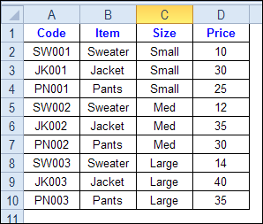
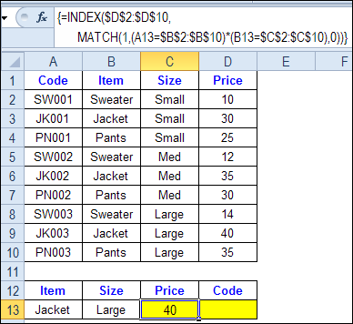
In the screen shot below, each item is listed 3 times in the pricing lookup table. We want to find the price for a large jacket.

在下面的屏幕快照中，每个商品在定价查询表中列出了3次。 我们想找到一件大外套的价格。

To get the right price, you'll need to use 2 criteria:

为了获得合适的价格，您需要使用两个条件：

• the item name
  项目名称
• the size
  规模

它匹配吗？ 对或错 (Does it MATCH? True or False)

Instead of a simple MATCH formula, we'll use one that checks both the Item and Size columns.

代替简单的MATCH公式，我们将使用一个检查Item和Size列的公式。

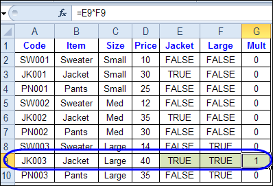
To see how this formula will work, I'll temporarily add columns to check the item and Size of each item -- is the item a Jacket, and is the Size a Large?

为了了解此公式的工作原理，我将临时添加列以检查项目和每个项目的大小-该项目是夹克，还是大尺寸？

Enter this formula in E2, and copy down to E10: =C2=$C$13

在E2中输入此公式，然后向下复制到E10： = C2 = $ C $ 13

Enter this formula in F2, and copy down to F10: =D2=$D$13

在F2中输入此公式，然后向下复制到F10： = D2 = $ D $ 13

• If the Item in column B is a Jacket, the result in column E is TRUE. If not, the result is FALSE
  如果B列中的项目是夹克，则E列中的结果为TRUE。 如果不是，则结果为FALSE
• If the Size in column C is Large, the result in column F is TRUE. If not, the result is FALSE
  如果C列中的Size为大，则F列中的结果为TRUE。 如果不是，则结果为FALSE

To see if both results are TRUE in each row, enter this formula in G2, and copy down to G10: =F2*G2

若要查看每行的两个结果是否均为TRUE，请在G2中输入此公式，然后向下复制到G10： = F2 * G2

When you multiply the TRUE/FALSE values,

当您将TRUE / FALSE值相乘时，

• If either value is FALSE (0), the result is zero
  如果任一值为FALSE(0)，则结果为零
• If both values are TRUE, the result is 1
  如果两个值均为TRUE，则结果为1

Only the 8th row  in our list of items has a 1, because both values are TRUE in that row.

在我们的商品列表中，只有第8行的数字为1，因为该行的两个值均为TRUE。

We can tell the MATCH function to look for a 1, and that will return the information that we need.

我们可以告诉MATCH函数寻找1 ，这将返回我们需要的信息。

将MATCH与多个条件一起使用 (Use MATCH With Multiple Criteria)

Instead of adding extra columns to the worksheet, we can use an array-entered INDEX and MATCH formula to do all the work.

无需在工作表中添加额外的列，我们可以使用输入数组的INDEX和MATCH公式来完成所有工作。

Here is the formula that we'll use to get the correct price, and the explanation is below:

这是我们用来获取正确价格的公式，解释如下：

=INDEX($D$2:$D$10, MATCH(1,(A13=$B$2:$B$10) * (B13=$C$2:$C$10),0))

= INDEX( $ D $ 2：$ D $ 10 ，MATCH(1，(A13 = $ B $ 2：$ B $ 10)*(B13 = $ C $ 2：$ C $ 10)，0))

NOTE: This is an array-entered formula, so press Ctrl + Shift + Enter, instead of just pressing the Enter key.

注意 ：这是一个数组输入的公式 ，因此请按Ctrl + Shift + Enter ，而不是仅按Enter键。

公式如何运作 (How the Formula Works)

In this INDEX and MATCH example,

在此INDEX和MATCH示例中，

• prices are in cells D2:D10, so that is the range that the INDEX function will use

  价格在单元格D2：D10中 ，所以这是INDEX函数将使用的范围

• the item name is in cell A13

  项目名称在单元格A13中

• the size is in cell B13.

  大小在单元格B13中 。

The formula checks for the selected items in $B$2:$B$10, and sizes in $C$2:$C$10. The results are multiplied.

该公式将检查$ B $ 2：$ B $ 10中的选定项目，并检查$ C $ 2：$ C $ 10中的大小 。 结果相乘。

• (A13=$B$2:$B$10)*(B13=$C$2:$C$10)

  ( A13 = $ B $ 2：$ B $ 10 )*( B13 = $ C $ 2：$ C $ 10 )

The MATCH function looks for the 1 in the array of results.

MATCH函数在结果数组中查找1 。

• MATCH(1,(A13=$B$2:$B$10)*(B13=$C$2:$C$10),0)

  MATCH(1，( A13 = $ B $ 2：$ B $ 10 )*( B13 = $ C $ 2：$ C $ 10 )，0)

If you select that part of the formula and press the F9 key, you can see the calculated results. In the screen shot below there are 9 results, and all are zero, except the 8th result, which is 1.

如果选择公式的该部分并按F9键，则可以看到计算的结果。 在下面的屏幕截图中，有9个结果，除第8个结果为1之外，其余均为零。

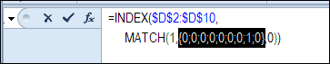
So, the INDEX function returns the price – 40 – from the 8th data row in column D (cell D9).

因此，INDEX函数从D列(单元格D9)的第8个数据行返回价格-40。

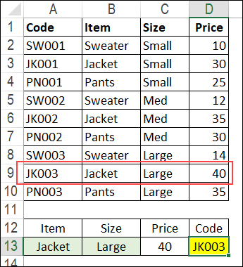
获取产品代码 (Get the Product Code)

To find the product code for the selected item and size, you would change the formula to look in cells A2:A10, instead of the price column.

要查找所选商品和尺寸的产品代码，您可以更改公式以在单元格A2：A10中查找，而不是在价格列中查找。

Put this formula in cell D13, and remember, this is an array-entered formula, so press Ctrl + Shift + Enter.

将此公式放在单元格D13中，请记住，这是一个数组输入的公式 ，因此请按Ctrl + Shift + Enter 。

=INDEX($A$2:$A$10, MATCH(1,(A13=$B$2:$B$10) * (B13=$C$2:$C$10),0))

= INDEX( $ A $ 2：$ A $ 10 ，MATCH(1，(A13 = $ B $ 2：$ B $ 10)*(B13 = $ C $ 2：$ C $ 10)，0))

In this example, the product code would be JK003, from cell A9.

在此示例中，产品代码为单元格A9中的JK003。

获取工作簿 (Get the Workbook)

To get the sample file with the Lookup Multiple Criteria examples, go to the Excel Lookup Multiple Criteria page on my Contextures site.

若要获取带有“查找多个条件”示例的示例文件，请转到Contextures网站上的“ Excel查找多个条件”页面 。

For more INDEX and MATCH tips and examples, visit the INDEX function and MATCH function page on the Contextures website. This is Example 4 in the sample file section of that page.

有关更多INDEX和MATCH提示和示例的信息，请访问Contextures网站上的INDEX函数和MATCH函数页面 。 这是该页面的示例文件部分中的示例4。

翻译自: https://contexturesblog.com/archives/2012/07/12/check-multiple-criteria-with-excel-index-and-match/