主要步骤和思路:
1.搭建tensorflow环境,导入需要用到的python库,比较简单,可自行百度。
2.从sklearn库中导入自带的鸢尾花数据集。
3.将数据集划分为训练集和测试集,训练集与测试集比例为8:2。
4.接下来需要一些tensorflow的基础知识,创建变量,定义模型,定义损失函数,定义优化方法等,然后开始训练。
5.训练完成之后,会保存训练出的模型,预测时读入模型进行预测即可。
下面附上代码
训练代码:train.py
# -- coding: utf-8 --

import matplotlib.pyplot as plt
import numpy as np
import tensorflow as tf
from sklearn import datasets

# 获取数据
iris = datasets.load_iris()
x_vals = np.array([[x[0], x[3]] for x in iris.data])
y_vals = np.array([1 if y == 0 else -1 for y in iris.target])

# 分离训练和测试集
train_indices = np.random.choice(len(x_vals),int(len(x_vals)*0.8),replace=False)
test_indices = np.array(list(set(range(len(x_vals))) - set(train_indices)))
x_vals_train = x_vals[train_indices]
x_vals_test = x_vals[test_indices]
y_vals_train = y_vals[train_indices]
y_vals_test = y_vals[test_indices]

batch_size = 100

# 初始化feed in
x_data = tf.placeholder(shape=[None, 2], dtype=tf.float32)
y_target = tf.placeholder(shape=[None, 1], dtype=tf.float32)

# 创建权值参数
A = tf.Variable(tf.random_normal(shape=[2, 1]))
b = tf.Variable(tf.random_normal(shape=[1, 1]))

# 定义线性模型: y = Ax + b
model_output = tf.subtract(tf.matmul(x_data, A), b)

# Declare vector L2 'norm' function squared
l2_norm = tf.reduce_sum(tf.square(A))

# Loss = max(0, 1-pred*actual) + alpha * L2_norm(A)^2
alpha = tf.constant([0.01])
classification_term = tf.reduce_mean(tf.maximum(0., tf.subtract(1., tf.multiply(model_output, y_target))))
loss = tf.add(classification_term, tf.multiply(alpha, l2_norm))

my_opt = tf.train.GradientDescentOptimizer(0.01)
train_step = my_opt.minimize(loss)

#持久化
saver = tf.train.Saver()

with tf.Session() as sess:
    init = tf.global_variables_initializer()
    sess.run(init)

# Training loop
    for i in range(20000):
        rand_index = np.random.choice(len(x_vals_train), size=batch_size)
        rand_x = x_vals_train[rand_index]
        rand_y = np.transpose([y_vals_train[rand_index]])
        sess.run(train_step, feed_dict={x_data: rand_x, y_target: rand_y})
    saver.save(sess, "./model/model.ckpt")
预测代码:predict.py
# -- coding: utf-8 --

import matplotlib.pyplot as plt
import numpy as np
import tensorflow as tf
from sklearn import datasets


# 获取数据
iris = datasets.load_iris()
x_vals = np.array([[x[0], x[3]] for x in iris.data])
y_vals = np.array([1 if y == 0 else -1 for y in iris.target])

# 分离训练和测试集
test_indices = np.random.choice(len(x_vals),int(len(x_vals)*0.8),replace=False)
x_vals_test = x_vals[test_indices]
y_vals_test = y_vals[test_indices]

# 初始化feed in
x_data = tf.placeholder(shape=[None, 2], dtype=tf.float32)
y_target = tf.placeholder(shape=[None, 1], dtype=tf.float32)

# 创建权值参数
A = tf.Variable(tf.random_normal(shape=[2, 1]))
b = tf.Variable(tf.random_normal(shape=[1, 1]))

# 定义线性模型: y = Ax + b
model_output = tf.subtract(tf.matmul(x_data, A), b)

#判断准确度
result = tf.maximum(0., tf.multiply(model_output, y_target))

saver = tf.train.Saver()

with tf.Session() as sess:
    saver.restore(sess, "./model/model.ckpt")
    y_test = np.reshape(y_vals_test, (120,1))
    array = sess.run(result, feed_dict={x_data: x_vals_test, y_target: y_test})
    num = np.array(array)
    zero_num = np.sum(num==[0])
    print(num)
    print(zero_num)
分类后数据可视化代码:plotdata.py
# -- coding: utf-8 --

import matplotlib.pyplot as plt
import numpy as np
import tensorflow as tf
from sklearn import datasets

# 获取数据
iris = datasets.load_iris()
#数据集
print(iris.data)
#类别标签
print(iris.target)
#特征名称
print(iris.feature_names)
#类别名称
print(iris.target_names)
#取了第一个特征和第4个特征
x_vals = np.array([[x[0], x[3]] for x in iris.data])
print(x_vals)
y_vals = np.array([1 if y == 0 else -1 for y in iris.target])

# 分离训练集和测试集
train_indices = np.random.choice(len(x_vals),int(len(x_vals)*0.8),replace=False)
test_indices = np.array(list(set(range(len(x_vals))) - set(train_indices)))
x_vals_train = x_vals[train_indices]
x_vals_test = x_vals[test_indices]
y_vals_train = y_vals[train_indices]
y_vals_test = y_vals[test_indices]

batch_size = 100

# 初始化feed in
x_data = tf.placeholder(shape=[None, 2], dtype=tf.float32)
y_target = tf.placeholder(shape=[None, 1], dtype=tf.float32)

# 创建权值参数
A = tf.Variable(tf.random_normal(shape=[2, 1]))
b = tf.Variable(tf.random_normal(shape=[1, 1]))

A2 = tf.Variable(tf.random_normal(shape=[2, 1]))
b2 = tf.Variable(tf.random_normal(shape=[1, 1]))

# 定义线性模型: y = Ax + b
model_output = tf.subtract(tf.matmul(x_data, A), b)
model_output2 = tf.subtract(tf.matmul(x_data, A2), b2)

# Declare vector L2 'norm' function squared
l2_norm = tf.reduce_sum(tf.square(A))

# Loss = max(0, 1-pred*actual) + alpha * L2_norm(A)^2
alpha = tf.constant([0.01])
classification_term = tf.reduce_mean(tf.maximum(0., tf.subtract(1., tf.multiply(model_output, y_target))))
classification_term2 = tf.reduce_mean(tf.maximum(0., tf.subtract(1., tf.multiply(model_output2, y_target))))
loss = tf.add(classification_term, tf.multiply(alpha, l2_norm))
loss2 = tf.add(classification_term2,[0])

my_opt = tf.train.GradientDescentOptimizer(0.01)
train_step = my_opt.minimize(loss)

my_opt2 = tf.train.GradientDescentOptimizer(0.01)
train_step2 = my_opt2.minimize(loss2)

with tf.Session() as sess:
    init = tf.global_variables_initializer()
    sess.run(init)

# Training loop
    loss_vec = []
    train_accuracy = []
    test_accuracy = []
    for i in range(20000):
        rand_index = np.random.choice(len(x_vals_train), size=batch_size)
        rand_x = x_vals_train[rand_index]
        rand_y = np.transpose([y_vals_train[rand_index]])
        sess.run(train_step, feed_dict={x_data: rand_x, y_target: rand_y})
        sess.run(train_step2, feed_dict={x_data: rand_x, y_target: rand_y})


    [[a1], [a2]] = sess.run(A)
    [[b]] = sess.run(b)
    slope = -a2/a1
    y_intercept = b/a1
    best_fit = []

    [[a12], [a22]] = sess.run(A2)
    [[b2]] = sess.run(b2)
    slope2 = -a22/a12
    y_intercept2 = b2/a12
    best_fit2 = []

    x1_vals = [d[1] for d in x_vals]

    for i in x1_vals:
     best_fit.append(slope*i+y_intercept)
     best_fit2.append(slope2*i+y_intercept2)


# Separate I. setosa
    setosa_x = [d[1] for i, d in enumerate(x_vals) if y_vals[i] == 1]
    setosa_y = [d[0] for i, d in enumerate(x_vals) if y_vals[i] == 1]
    not_setosa_x = [d[1] for i, d in enumerate(x_vals) if y_vals[i] == -1]
    not_setosa_y = [d[0] for i, d in enumerate(x_vals) if y_vals[i] == -1]

    plt.plot(setosa_x, setosa_y, 'o', label='I. setosa')
    plt.plot(not_setosa_x, not_setosa_y, 'x', label='Non-setosa')
    plt.plot(x1_vals, best_fit, 'r-', label='Linear Separator + w', linewidth=3)
    plt.plot(x1_vals, best_fit2, 'r-', label='Linear Separator', color='b', linewidth=3)
    plt.ylim([0, 10])
    plt.legend(loc='lower right')
    plt.title('Sepal Length vs Pedal Width')
    plt.xlabel('Pedal Width')
    plt.ylabel('Sepal Length')
    plt.show()
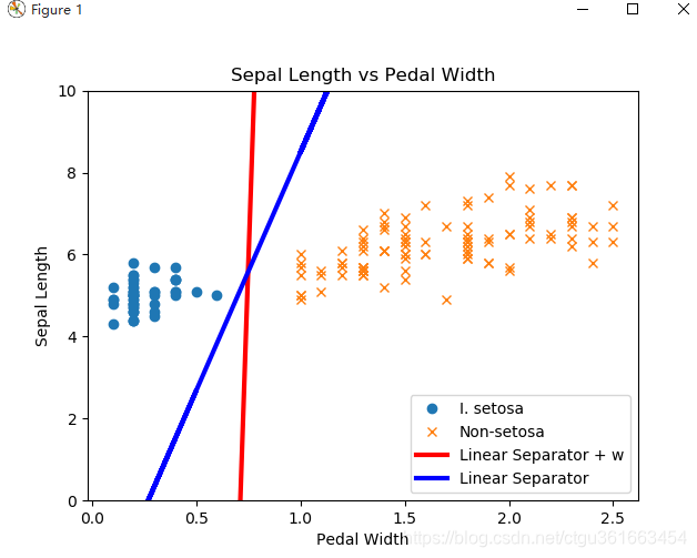
分类结果:
注意,这里是线性分类,只分成了两类,setosa类和非setosa类,数据集中的鸢尾花是有三种类别setosa, versicolor ,virginica。


 本文介绍如何使用TensorFlow对鸢尾花数据集进行线性分类,包括环境搭建、数据预处理、模型训练及预测,并提供训练、预测和数据可视化的完整代码。


 1341
1341

 被折叠的 条评论
为什么被折叠?
被折叠的 条评论
为什么被折叠?
 到【灌水乐园】发言


