mport numpy as np
import ufl
# 正确的UFL元素导入方式(适配UFL 2023+,兼容DOLFINx 0.6+)
from ufl.finiteelement import FiniteElement, MixedElement
from ufl import finiteelement
ve = finiteelement.VectorElement(...)
from dolfinx import mesh, fem, io
from mpi4py import MPI
import numpy as np
from mpi4py import MPI
from petsc4py import PETSc
from dolfinx import fem, mesh, plot
from dolfinx.io import XDMFFile
import matplotlib.pyplot as plt
# ------------------------------------------------------
# 1. 材料与几何参数
# ------------------------------------------------------
E = 2e11 # 弹性模量 (Pa)
nu = 0.3 # 泊松比
h = 0.01 # 板厚 (m)
L, W = 2.0, 2.0 # 板尺寸 (m)
q = 1000 # 均布荷载 (N/m²)
# ------------------------------------------------------
# 2. 本构矩阵与Q阵
# ------------------------------------------------------
D_mat = E / ((1 + nu) * (1 - 2 * nu))
Ce = D_mat * np.array([[1 - nu, 0, nu],
[0, (1 - 2*nu)/2, 0],
[nu, 0, 1 - nu]], dtype=np.float64)
Cet = D_mat * np.array([[0, 0, nu],
[0, 0, 0],
[0, 0, nu]], dtype=np.float64)
Ct = D_mat * np.array([[(1 - 2*nu)/2, 0, 0],
[0, (1 - 2*nu)/2, 0],
[0, 0, 1 - nu]], dtype=np.float64)
Ct_inv = np.linalg.inv(Ct)
Q = Ce - Cet @ Ct_inv @ Cet.T
# ABD刚度矩阵
A = Q * h
B = Q * (h**2 / 2)
D = Q * (h**3 / 12)
ABD = np.block([[A, B], [B.T, D]])
# ------------------------------------------------------
# 3. 网格与混合函数空间(核心修正:统一e和k的空间)
# ------------------------------------------------------
domain = mesh.create_rectangle(
MPI.COMM_WORLD,
[[0.0, 0.0], [L, W]],
[20, 20],
mesh.CellType.quadrilateral
)
# 定义e(3分量)和k(3分量)的混合元素
element_e = VectorElement("Lagrange", domain.ufl_cell(), 2, dim=3) # e = [e11, e22, e12]
element_k = VectorElement("Lagrange", domain.ufl_cell(), 2, dim=3) # k = [k11, k22, k12]
mixed_element = MixedElement([element_e, element_k]) # 混合元素:(e, k)
V = fem.FunctionSpace(domain, mixed_element) # 统一的混合函数空间
# 定义混合空间中的trial和test函数
(e, k) = ufl.TrialFunctions(V) # 解变量:e和k
(e_test, k_test) = ufl.TestFunctions(V) # 测试变量
# 组合向量:[e11, e22, e12, k11, k22, k12]
vec = ufl.as_vector([e[0], e[1], e[2], k[0], k[1], k[2]])
vec_test = ufl.as_vector([e_test[0], e_test[1], e_test[2], k_test[0], k_test[1], k_test[2]])
# ------------------------------------------------------
# 4. 变分形式(修正:基于混合空间)
# ------------------------------------------------------
# 应变能
energy = 0.5 * ufl.inner(vec, ufl.as_matrix(ABD) @ vec) * ufl.dx
# 外力功(均布荷载,作用于弯曲部分)
W_ext = q * ufl.inner(k, ufl.as_vector([0, 1, 0])) * ufl.dx # 与k22耦合
# 变分方程
a = fem.form(ufl.derivative(energy, (e, k), (e_test, k_test)))
L_form = fem.form(ufl.derivative(W_ext, (e, k), (e_test, k_test)))
# ------------------------------------------------------
# 5. 边界条件(修正:针对混合空间的子空间)
# ------------------------------------------------------
def boundary_simply_supported(x):
return (np.isclose(x[0], 0.0) | np.isclose(x[0], L) |
np.isclose(x[1], 0.0) | np.isclose(x[1], W))
# 面内应变e的边界条件:e=0(针对混合空间的第0个子空间)
V_e_sub = V.sub(0) # e所在的子空间
V_e_sub_dofmap = V_e_sub.dofmap
dofs_e = fem.locate_dofs_geometrical((V_e_sub, V_e_sub_dofmap), boundary_simply_supported)
bc_e = fem.dirichletbc(PETSc.ScalarType(0), dofs_e, V_e_sub)
bcs = [bc_e]
# ------------------------------------------------------
# 6. 求解(修正:解属于混合空间)
# ------------------------------------------------------
sol = fem.Function(V) # 混合空间的解:包含e和k
problem = fem.petsc.LinearProblem(
a, L_form, bcs=bcs,
petsc_options={"ksp_type": "preonly", "pc_type": "lu"}
)
sol = problem.solve()
# 拆分e和k的解(从混合空间提取)
e_sol = sol.sub(0).collapse() # 面内应变
k_sol = sol.sub(1).collapse() # 曲率
e_sol.name = "In-plane Strain e"
k_sol.name = "Curvature k"
# ------------------------------------------------------
# 7. 应力计算
# ------------------------------------------------------
x3_top = h / 2
eps_total = ufl.as_vector([
e_sol[0] + x3_top * k_sol[0],
e_sol[1] + x3_top * k_sol[1],
e_sol[2] + x3_top * k_sol[2],
0, 0, 0
])
C_full = np.block([[Ce, Cet], [Cet.T, Ct]])
sigma = ufl.dot(ufl.as_matrix(C_full), eps_total)
sigma_11 = sigma[0]
sigma_22 = sigma[1]
# 插值到可视化空间
V_sigma = fem.FunctionSpace(domain, ("Lagrange", 1))
sigma_11_func = fem.Function(V_sigma)
sigma_11_func.interpolate(fem.Expression(sigma_11, V_sigma.element.interpolation_points()))
sigma_22_func = fem.Function(V_sigma)
sigma_22_func.interpolate(fem.Expression(sigma_22, V_sigma.element.interpolation_points()))
# ------------------------------------------------------
# 8. 可视化
# ------------------------------------------------------
# 8.1 面内应变e11
fig1, ax1 = plt.subplots(figsize=(8, 6))
plot.plot_scalar_field(e_sol.sub(0), title="In-plane Strain e11", ax=ax1, cmap="viridis")
plt.colorbar(ax1.collections[0], ax=ax1)
plt.show()
# 8.2 曲率k11
fig2, ax2 = plt.subplots(figsize=(8, 6))
plot.plot_scalar_field(k_sol.sub(0), title="Curvature k11", ax=ax2, cmap="coolwarm")
plt.colorbar(ax2.collections[0], ax=ax2)
plt.show()
# 8.3 应力σ11
fig3, ax3 = plt.subplots(figsize=(8, 6))
plot.plot_scalar_field(sigma_11_func, title="Stress σ11 (Pa)", ax=ax3, cmap="plasma")
plt.colorbar(ax3.collections[0], ax=ax3)
plt.show()
# 8.4 应力σ22
fig4, ax4 = plt.subplots(figsize=(8, 6))
plot.plot_scalar_field(sigma_22_func, title="Stress σ22 (Pa)", ax=ax4, cmap="jet")
plt.colorbar(ax4.collections[0], ax=ax4)
plt.show()
# 保存结果
with XDMFFile(domain.comm, "e_k_sigma_results.xdmf", "w") as file:
file.write_mesh(domain)
file.write_function(e_sol)
file.write_function(k_sol)
file.write_function(sigma_11_func)
file.write_function(sigma_22_func)


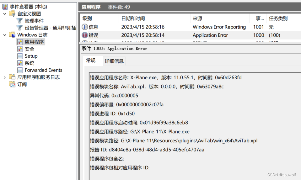
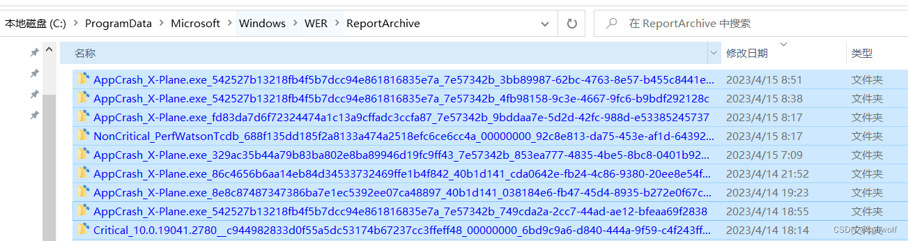
 博主的X-Plane APP崩溃且无警告,通过事件查看器找到目录【C:\\ProgramData\\Microsoft\\Windows\\WER\\ReportArchive】,发现Windows记录了每一次APP崩溃的原因。
 6910
6910

 被折叠的 条评论
为什么被折叠?
被折叠的 条评论
为什么被折叠?
 到【灌水乐园】发言


