Shoelace formula

最新推荐文章于 2025-03-08 08:27:35 发布

转载最新推荐文章于 2025-03-08 08:27:35 发布 · 2.3k 阅读

文章标签：

#numbers #algorithm #equals #matrix #variables #each

数学知识专栏收录该内容

8 篇文章

订阅专栏

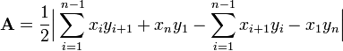
本文介绍了一种用于计算简单多边形面积的数学算法——鞋带公式。该算法通过交叉相乘坐标来确定多边形所包围的面积，并从周围多边形中减去这部分面积以得到内部多边形的面积。文章提供了详细的计算步骤和实例。

From Wikipedia, the free encyclopedia

The shoelace formula, or shoelace algorithm, is a mathematical algorithm to determine the area of a simple polygon whose vertices are described by ordered pairs in the plane^[1]. The user cross-multiplies corresponding coordinates to find the area encompassing the polygon, and subtracts it from the surrounding polygon to find the area of the polygon within. It is called the shoelace formula because of the constant cross-multiplying for the coordinates making up the polygon, like tying shoelaces^[2]. It is also sometimes called the shoelace method. It is also known as Gauss' area formula, after Carl Friedrich Gauss. It has applications in surveying and forestry,^[3] among other areas. It is also called the surveyor's formula^[4].

The formula can be represented by the expression:

$\mathbf{A} = {1 \over 2} \Big | \sum_{i=1}^{n-1} x_iy_{i+1} + x_ny_1 - \sum_{i=1}^{n-1} x_{i+1}y_i - x_1y_n \Big |$

$= {1 \over 2}|x_1y_2 + x_2y_3 + \cdots + x_{n-1}y_n + x_ny_1 - x_2y_1 - x_3y_2 - \cdots - x_ny_{n-1} - x_1y_n|$

where

A is the area of the polygon,
n is the number of sides of the polygon, and
(x_i, y_i), i = 1, ,..., n are the vertices (or "corners") of the polygon.^[5]

Alternatively:^[3]^[6]

$\mathbf{A} = {1 \over 2} \Big | \sum_{i=1}^{n} x_i(y_{i+1}-y_{i-1}) \Big | = {1 \over 2} \Big | \sum_{i=1}^{n} y_i(x_{i+1}-x_{i-1}) \Big | = {1 \over 2} \Big | \sum_{i=1}^{n} x_iy_{i+1}-x_{i+1}y_i \Big |$

where x_n+1 = x₁ and x₀ = x_n, as well as y_n+1 = y₁ and y₀ = y_n.

If the points are labeled sequentially in the counterclockwise direction, then the above determinants are positive and the absolute value signs can be omitted;^[4] if they are labeled in the clockwise direction, the determinants will be negative. This is because the formula can be viewed as a special case of Green's Theorem.

[hide]

[edit] Examples

The user must know the points of the polygon in a Cartesian plane. For example, take a triangle with coordinates {(2, 1), (4, 5), (7, 8)}. Take the first x-coordinate and multiply it by the second y-value, and repeat, and keep repeating this process. This can be defined by this formula:

$\mathbf{A}_\text{tri.} = {1 \over 2}|x_1y_2 + x_2y_3 + x_3y_1 - x_2y_1 - x_3y_2 - x_1y_3|$

for x_n and y_n representing each respective coordinate. This formula is just the expansion of those given above for the case n = 3. Using it, one can find that the area of the triangle equals one half of the absolute value of 10 + 32 + 7 − 4 − 35 − 16, which equals 3. The number of variables depends on the number of sides of the polygon. For example, a pentagon will be defined up to x₅ and y₅:

$\mathbf{A}_\text{pent.} = {1 \over 2}|x_1y_2 + x_2y_3 + x_3y_4 + x_4y_5 + x_5y_1 - x_2y_1 - x_3y_2 - x_4y_3 - x_5y_4 - x_1y_5|$

A quadrilateral will be defined up to x₄ and y₄:

$\mathbf{A}_\text{quad.} = {1 \over 2}|x_1y_2 + x_2y_3 +x_3y_4 + x_4y_1 - x_2y_1 - x_3y_2 - x_4y_3 - x_1y_4|$

[edit] More complex example

Consider the polygon defined by the points (3,4), (5,11), (12,8), (9,5), and (5,6), and illustrated in the following diagram:

The area of this polygon is:

$\begin{align}\mathbf{A} & = {1 \over 2}|3 \times 11 + 5 \times 8 + 12 \times 5 + 9 \times 6 + 5 \times 4 \\& {} \qquad\qquad {} - 4 \times 5 - 11 \times 12 - 8 \times 9 - 5 \times 5 - 6 \times 3| \\[10pt]& = {60 \over 2} = 30\end{align}$

[edit] Explanation of name

The reason this formula is called the shoelace formula is because of a common method used to evaluate it. This method uses matrices. As an example, choose the triangle with vertices (2,4), (3,−8), and (1,2). Then construct the following matrix by “walking around” the triangle and ending with the initial point.

$\begin{bmatrix} 2 & 4 \\ 3 & -8 \\ 1 & 2 \\ 2 & 4 \end{bmatrix}$ ^[7]

First, draw diagonal down and to the right slashes (as shown below),

and multiply the two numbers connected by each slash, then add all the products: (2 × −8) + (3 × 2) + (1 × 4) = −6. Do the same with slashes diagonal down and to the left (shown below with former slashes):

(4 × 3) + (−8 × 1) + (2 × 2) = 8. Then, subtract these two numbers and take the absolute value of the difference: |−6 − 8| = 14. Halving this gives the area of the triangle: 7. Organizing the numbers like this makes the formula easier to recall and evaluate. With all the slashes drawn, the matrix loosely resembles a shoe with the laces done up, giving rise to the algorithm's name.