【Fast RCNN】《Fast-RCNN》

原创已于 2024-06-06 14:11:39 修改 · 541 阅读

1 ·

CC 4.0 BY-SA版权

文章标签：

#深度学习 #目标检测 #计算机视觉 #fast rcnn #人工智能

于 2018-08-08 16:23:40 首次发布

CNN / Transformer 专栏收录该内容

254 篇文章

订阅专栏

Fast R-CNN是一种高效的目标检测算法，相比R-CNN和SPPnet，它实现了end-to-end的训练，提升了检测速度和精度。通过多任务损失、RoI池化层、预训练网络初始化等创新，Fast R-CNN解决了传统方法的多阶段训练问题。

摘要生成于 C知道，由 DeepSeek-R1 满血版支持，前往体验 >

这里写图片描述

ICCV2015

1 Motivation

Compared to image classification, object detection is a more challenging task that requires more complex methods to solve. Due to this complexity, current approaches train models in multi-stage pipelines that are slow and inelegant.

Fast R-CNN employs several innovations to improve training and testing speed while also increasing detection accuracy.

Innovation

multi-task loss
ROI pooling

这里写图片描述

2 Drawbacks of R-CNN and SPPnet

Training is a multi-stage pipeline（proposal、classification、bbox regression，改进Multi-task loss）
Training is expensive in space and time（要从每一张图像上提取大量proposal，还要从每个proposal中提取特征，并存到磁盘中）
Object detection is slow.

3 Advantages

Higher detection quality (mAP) than R-CNN, SPPnet
Training is single-stage, using a multi-task loss
Training can update all network layers
No disk storage is required for feature caching

4 Method

这里写图片描述

Conv → ROI pooling → FC → softmax/bbox regression

4.1 The RoI pooling layer

【ROI Pooling】Region of interest pooling

这样做有下面几个好处：

统一输出维度，这个是必须的。
相比于SPP-Net，RoI pooling的维度更少，假设RoI pooling选择了4*4的话，那么维度就可以从21个bin（16+4+1）降低为16个，虽然这样看来降低的并不多，但是不要忘了特征还有厚度，如果厚度是256的话，那么降维就比较可观了。
RoI pooling不再是多尺度的池化，这样一来梯度回传就会更方便，有利于Fast R-CNN 实现 end-to-end 的训练。

这里详细补充下 RoI Pooling 的细节！就是 bin 到底怎么划分的！下面我们看看每个 bin 处理的源码！
在这里插入图片描述
假设目标大小是正方形 $36 * 36$ (0-35)，要池化成 $5 * 5$ ，我们分析 $h$ 或者 $w$ 一个维度就好了！

roi_width = 35-0+1 = 36
bin_size_h = 36/5 = 7.2
ph 是索引，取 0~4

我们可以推算出每个 bin 的 $h$ 维度取值范围（左开右闭，代码中没有截取出来）

$\sim ceil(7.2*1) = [0,8) = [0,7]$
$\sim ceil(7.2*2) = [7,15) = [7,14]$
$\sim ceil(7.2*3)= [14,22) = [14,21]$
$\sim ceil(7.2*4) = [21,29) = [21,28]$
$\sim ceil(7.2*5)= [28,36) = [28,35]$

区间长度是 8，8，8，8，8，四个像素的重叠 40-4 = 36

再来个例子

假设目标大小是正方形 $39 * 39$ (0-38)，要池化成 $5 * 5$ ，我们分析 $h$ 或者 $w$ 一个维度就好了！

roi_width = 38-0+1 = 39
bin_size_h = 39/5 = 7.8
ph 是索引，取 0~4

我们可以推算出每个 bin 的 $h$ 维度取值范围（左开右闭，代码中没有截取出来）

$\sim ceil(7.8*1) = [0,8) = [0,7]$
$\sim ceil(7.8*2) = [7,16) = [7,15]$
$\sim ceil(7.8*3)= [15,24) = [14,23]$
$\sim ceil(7.8*4) = [23,32) = [23,31]$
$\sim ceil(7.8*5)= [31,39) = [31,38]$

区间长度是 8，9，9，9，8，四个像素的重叠 43-4 = 39

总结：RoI Pooling 划分 bin 的方式是，有重叠的，不等分的，无剩余的划分！！！

4.2 Initializing from pretrained networks

用了3个预训练的ImageNet网络（CaffeNet/VGG_CNN_M_1024/VGG16）。
预训练的网络初始化Fast RCNN要经过三次变形：

最后一个max pooling层替换为RoI pooling层，设置H’和W’与第一个全连接层兼容。
(SPPnet for one scale -> arbitrary input image size )
最后一个全连接层和softmax（原本是1000个类）-> 替换为softmax的对K+1个类别的分类层，和bounding box 回归层。
(Cls and Det at same time)
输入修改为两种数据：一组N（batch size）个图形，R个RoI，batch size和ROI数、图像分辨率都是可变的。

4.3 Finetuning for detection

前面说过SPPnet有一个缺点是只能微调spp层后面的全连接层，所以SPPnet就可以采用随机梯度下降（SGD）来训练。
RCNN:无法同时tuning在SPP layer两边的卷积层和全连接层
RoI-centric sampling：从所有图片的所有RoI中均匀取样，这样每个SGD的mini-batch中包含了不同图像中的样本。（SPPnet采用）
FRCN想要解决微调的限制,就要反向传播到spp层之前的层->(reason)反向传播需要计算每一个RoI感受野的卷积层，通常会覆盖整个图像，如果一个一个用RoI-centric sampling的话就又慢又耗内存。

Fast RCNN:->改进了SPP-Net在实现上无法同时tuning在SPP layer两边的卷积层和全连接层

image-centric sampling： (solution)mini-batch采用层次取样，先对图像取样，再对RoI取样，同一图像的RoI共享计算和内存。

另外，FRCN在一次微调中联合优化softmax分类器和bbox回归。
看似一步，实际包含了：
多任务损失（multi-task loss）、小批量取样（mini-batch sampling）、RoI pooling层的反向传播（backpropagation through RoI pooling layers）、SGD超参数（SGD hyperparameters）。

4.3.1 efficient training method

原来128个 ROI 找128个图，现在minibatch为 N （eg：2），找 N 张图，每张图 R/N 个 ROI，eg： R = 128，N = 2，速度提升64倍
the proposed training scheme is roughly 64× faster than sampling one RoI from 128 different images (i.e., the R-CNN and SPPnet strategy).

这里写图片描述

4.3.2 Multi-task loss

这里写图片描述

$p$ 是softmax输出的类别的概率
$u$ 是类别的 ground truth
$\lambda$ hyper parameters
[u ≥ 1] evaluates to 1 when u ≥ 1 and 0 otherwise（0是background）
$t^u$ 是预测 $u$ 类别的 bbox 的 offset, $t^u = (t_x^u,t_y^u,t_w^u,t_h^u)$
v 是 ground truth 的 offset
$L_{cls}(p,u) = -logp_u$ ，log loss

这里写图片描述

蓝色的是x的平方

make the learning more robust against outliers

4.3.3 Mini-batch sampling

N张完整图片以50%概率水平翻转。
R个候选框的构成方式如下：
与 ground truth 25% IoU 0.5~1
与 ground truth 75% IoU [0.5,0.3)

4.3.4 Back-propagation through RoI pooling layers

这里写图片描述

简化下

RoI pooling层计算损失函数对每个输入变量x的偏导数，如下：

y 是 pooling 后的输出单元，x 是 pooling 前的输入单元，如果 y 由 x pooling而来，则将损失 L 对 y 的偏导计入累加值，最后累加完 R 个 RoI 中的所有输出单元。下面是我理解的 x、y、r 的关系：

Note：
RoI pooling是单层的SPP，也就是只用一层金字塔并在区域内做Max pooling，所以如何说在卷积层上提取特征的时候，特征的位置没有出现重叠，RoI pooling就是一个Max pooling，梯度回传也是一样的，而出现位置重叠的时候，梯度回传才会发生变化。

例如下面两张图，左边目标重叠了，右边目标没有重叠
这里写图片描述

显然，重叠的区域经过相同的坐标变换之后在卷积特征图上同样是有重叠的，那么这部分重叠的像素梯度应该如何让计算呢？ 是多个区域的偏导之和：
这里写图片描述

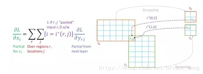
上图中有 r0 与 r1 两个区域，每个区域都通过 RoI pooling 之后生成4个bin， $x_{23}$ 的意思是第23个像素，那么计算 $x_{23}$ 位置的梯度就可以根据上图中左侧的公式，其中r是包含有这一点的区域，j是某个区域内的所有位置。
但是 $x_{23}$ 的梯度计算显然不需要r0，r1内的所有位置的梯度信息，它只需要包含 $x_{23}$ 这一点的，或者说是 $x_{23}$ 这一点有贡献的点的梯度，所以这里需要一个阈值函数 $i * (r, j)$ ，它的作用就是如果需要 RoI pooling 后的这一点的梯度，那么 $i * (r, j) = 1$ ，否则 $i * (r, j) = 0$ 。

这样一来，RoI pooling层的梯度回传只需要在 Max pooling 上简单修改即可。

4.4 Scale invariance

brute force（resize一样大）
using image pyramid

4.5 Truncated SVD for faster detection

在 fc6 和 fc7处用了SVD，mAP 只下降一点点，但是速度提升很多

25088×4096 matrix in VGG16’s fc6 layer
4096×4096 fc7 layer

Further speed-ups are possible with smaller drops in mAP if one fine-tunes again after compression.

5 训练和测试流程

这里写图片描述
在这里插入图片描述
图片参考微信公众号

6 Experiments and Conclusions

6.1 VOC2007、VOC2010、VOC2012 results

这里写图片描述

6.2 Training and testing time

CaffeNet as model S
VGG_CNN_M_1024 as M
VGG16 as L

这里写图片描述

6.3 Which layer to fine-tune？

这里写图片描述

Does this mean that all conv layers should be fine-tuned?
In short, no. In the smaller networks (S and M)，allowing conv1 to learn, or not, has no meaningful effect on mAP.

For VGG16（L）, we found it only necessary to update layers from conv3 1 and up (9 of the 13 conv layers).

7 Design evaluation

7.1. Does multitask training help?

yes
这里写图片描述

7.2 Scale invariance: to brute force or finesse?

brute force
这里写图片描述

scales 1 是 brute force，5 是 image pyramid，VGG（L） 5 会 out of memory

7.3 Do we need more training data?

table 1

7.4 Do SVMs outperform softmax?

no
这里写图片描述

7.5 Are more proposals always better?

no
这里写图片描述

8 总结

那么为什么Fast R-CNN比SPP-Net更快呢，最重要的原因就是 end-to-end 的训练，这样训练不再是分阶段的。

整个图像上仅运行一个CNN 而不是在超过2000 个重叠区域运行 2000 个CNN（根据网络的最后一层特征映射，而不是从原始图像本身生成区域提议）
softmax 代替 SVM（不用许多 SVM ）

缺点
虽然上面那张图上写的，Fast R-CNN的单图测试时间为0.32s，但是其实这样说并不准确，0.32为了和R-CNN的47.0s做对比。是的Fast R-CNN依然没有脱离ss算法，但是ss算法跑一张图的时间，大概是2s，所以讲道理的话，Fast R-CNN依然是达不到实时检测的要求的，好在ss算法在Faster R-CNN中被换成RPN（区域建议网络），这个我们后面再说。