


import numpy as np
import pandas as pd
from pandas import Series, DataFrame
movie = pd.read_excel('./tests.xlsx', sheet_name=1)
movie| 电影名称 | 武打镜头 | 接吻镜头 | 分类情况 | |
|---|---|---|---|---|
| 0 | 大话西游 | 36 | 1 | 动作片 |
| 1 | 杀破狼 | 43 | 2 | 动作片 |
| 2 | 前任3 | 0 | 10 | 爱情片 |
| 3 | 战狼2 | 59 | 1 | 动作片 |
| 4 | 泰坦尼克号 | 1 | 15 | 爱情片 |
| 5 | 星语心愿 | 2 | 19 | 爱情片 |
# 首先对于机器学习来说,字符串不代表可用数据,要么转成整数映射类型,要么不用
# X_train 表示的是要训练的数据
X_train = movie.iloc[:,1:-1]
# 答案
y_train = movie.iloc[:,-1:]
display(X_train, y_train)| 武打镜头 | 接吻镜头 | |
|---|---|---|
| 0 | 36 | 1 |
| 1 | 43 | 2 |
| 2 | 0 | 10 |
| 3 | 59 | 1 |
| 4 | 1 | 15 |
| 5 | 2 | 19 |
| 分类情况 | |
|---|---|
| 0 | 动作片 |
| 1 | 动作片 |
| 2 | 爱情片 |
| 3 | 动作片 |
| 4 | 爱情片 |
| 5 | 爱情片 |
# 引入机器学习的包
from sklearn.neighbors import KNeighborsClassifier
# n_neighbors默认值是5个,5个周围的样本
knn = KNeighborsClassifier(n_neighbors=5)
# 开始训练
knn.fit(X_train, y_train)
输出
KNeighborsClassifier(algorithm=’auto’, leaf_size=30, metric=’minkowski’,
metric_params=None, n_jobs=1, n_neighbors=5, p=2,
weights=’uniform’)
# 测试集
new_movie = DataFrame(np.array([['千星之城', 50, 10],['僵尸叔叔', 100, 2], ['超时空同居', 1, 12],['午夜凶铃', 0, 0]])
                     ,columns = ['电影名称', '武打镜头', '接吻镜头'])
new_movie| 电影名称 | 武打镜头 | 接吻镜头 | |
|---|---|---|---|
| 0 | 千星之城 | 50 | 10 |
| 1 | 僵尸叔叔 | 100 | 2 |
| 2 | 超时空同居 | 1 | 12 |
| 3 | 午夜凶铃 | 0 | 0 |
# 切片, 拿走没用的数据,比如电影名称
X_test = new_movie.iloc[:,1:]
X_test| 武打镜头 | 接吻镜头 | |
|---|---|---|
| 0 | 50 | 10 |
| 1 | 100 | 2 |
| 2 | 1 | 12 |
| 3 | 0 | 0 |
# 开始预测数据
y_test = knn.predict(X_test)
y_target = Series(y_test, name='分类情况')
y_target
输出
0 动作片
1 动作片
2 爱情片
3 爱情片
Name: 分类情况, dtype: object
data1 = pd.concat([new_movie, y_target], axis=1)
data1| 电影名称 | 武打镜头 | 接吻镜头 | 分类情况 | |
|---|---|---|---|---|
| 0 | 千星之城 | 50 | 10 | 动作片 |
| 1 | 僵尸叔叔 | 100 | 2 | 动作片 |
| 2 | 超时空同居 | 1 | 12 | 爱情片 |
| 3 | 午夜凶铃 | 0 | 0 | 爱情片 |
data = pd.concat([movie, data1],ignore_index = True)
data| 电影名称 | 武打镜头 | 接吻镜头 | 分类情况 | |
|---|---|---|---|---|
| 0 | 大话西游 | 36 | 1 | 动作片 |
| 1 | 杀破狼 | 43 | 2 | 动作片 |
| 2 | 前任3 | 0 | 10 | 爱情片 |
| 3 | 战狼2 | 59 | 1 | 动作片 |
| 4 | 泰坦尼克号 | 1 | 15 | 爱情片 |
| 5 | 星语心愿 | 2 | 19 | 爱情片 |
| 6 | 千星之城 | 50 | 10 | 动作片 |
| 7 | 僵尸叔叔 | 100 | 2 | 动作片 |
| 8 | 超时空同居 | 1 | 12 | 爱情片 |
| 9 | 午夜凶铃 | 0 | 0 | 爱情片 |
# 估测当前分类的准确值
y = Series(np.array(['动作片', '动作片', '爱情片', '动作片']), name='分类情况')
knn.score(X_test, y)
输出
0.75
1、k-近邻算法原理
简单地说,K-近邻算法采用测量不同特征值之间的距离方法进行分类。
- 优点:精度高、对异常值不敏感、无数据输入假定。
- 缺点:时间复杂度高、空间复杂度高。
- 适用数据范围:数值型和标称型。
工作原理
存在一个样本数据集合,也称作训练样本集,并且样本集中每个数据都存在标签,即我们知道样本集中每一数据
与所属分类的对应关系。输人没有标签的新数据后,将新数据的每个特征与样本集中数据对应的
特征进行比较,然后算法提取样本集中特征最相似数据(最近邻)的分类标签。一般来说,我们
只选择样本数据集中前K个最相似的数据,这就是K-近邻算法中K的出处,通常*K是不大于20的整数。
最后 ,选择K个最相似数据中出现次数最多的分类,作为新数据的分类*。
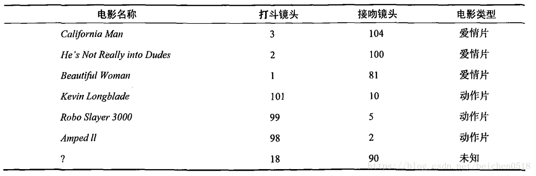
回到前面电影分类的例子,使用K-近邻算法分类爱情片和动作片。有人曾经统计过很多电影的打斗镜头和接吻镜头,下图显示了6部电影的打斗和接吻次数。假如有一部未看过的电影,如何确定它是爱情片还是动作片呢?我们可以使用K-近邻算法来解决这个问题。
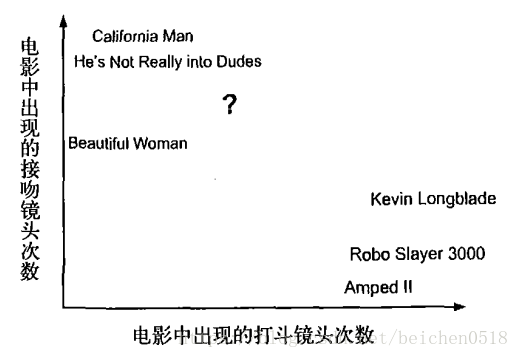
首先我们需要知道这个未知电影存在多少个打斗镜头和接吻镜头,上图中问号位置是该未知电影出现的镜头数图形化展示,具体数字参见下表。
即使不知道未知电影属于哪种类型,我们也可以通过某种方法计算出来。首先计算未知电影与样本集中其他电影的距离,如图所示。

现在我们得到了样本集中所有电影与未知电影的距离,按照距离递增排序,可以找到K个距
离最近的电影。假定k=3,则三个最靠近的电影依次是California Man、He’s Not Really into Dudes、Beautiful Woman。K-近邻算法按照距离最近的三部电影的类型,决定未知电影的类型,而这三部电影全是爱情片,因此我们判定未知电影是爱情片。
欧几里得距离(Euclidean Distance)
欧氏距离是最常见的距离度量,衡量的是多维空间中各个点之间的绝对距离。公式如下:

2、在scikit-learn库中使用k-近邻算法
分类问题:from sklearn.neighbors import KNeighborsClassifier
回归问题:from sklearn.neighbors import KNeighborsRegressor
0)一个最简单的例子
我们根据身高、体重、鞋子尺码数据分析性别
# 给机器学习的数据必须是二维的
X_train = np.array([[180, 80, 44], [165, 45, 38], [162, 40, 36], [170, 82, 42], [170, 52, 40], [175, 67, 42]])
# 目标值是一维的数据
y_train = np.array(['男', '女', '女', '男','女', '男'])
#先机器学习
knn.fit(X_train, y_train)输出
KNeighborsClassifier(algorithm=’auto’, leaf_size=30, metric=’minkowski’,
metric_params=None, n_jobs=1, n_neighbors=5, p=2,
weights=’uniform’)
# 定义预测的数据
X_test = np.array([[174, 72, 43], [163, 50, 38], [190, 80, 46]])
y = np.array(['男', '女', '女'])
# 开始预测
y_test = knn.predict(X_test)
y_test输出
array([‘男’, ‘女’, ‘男’], dtype=’
knn.score(X_test, y)输出
0.6666666666666666
把上面的数据转换成dataframe的
X_train_df = DataFrame(X_train, columns=['身高', '体重', '鞋码'])
y_train_df = DataFrame(y_train, columns=['性别'])
# 先学习
knn.fit(X_train_df, y_train_df)
KNeighborsClassifier(algorithm='auto', leaf_size=30, metric='minkowski',
metric_params=None, n_jobs=1, n_neighbors=5, p=2,
weights='uniform')
knn.predict(X_test)输出
array([‘男’, ‘女’, ‘男’], dtype=object)
鸢尾花识别
1)用于分类
导包,机器学习的算法KNN、数据蓝蝴蝶
import sklearn.datasets as datasetsiris = datasets.load_iris()
iris输出
{‘DESCR’: ‘Iris Plants Database\n====================\n\nNotes\n—–\nData Set Characteristics:\n :Number of Instances: 150 (50 in each of three classes)\n :Number of Attributes: 4 numeric, predictive attributes and the class\n :Attribute Information:\n - sepal length in cm\n - sepal width in cm\n - petal length in cm\n - petal width in cm\n - class:\n - Iris-Setosa\n - Iris-Versicolour\n - Iris-Virginica\n :Summary Statistics:\n\n ============== ==== ==== ======= ===== ====================\n Min Max Mean SD Class Correlation\n ============== ==== ==== ======= ===== ====================\n sepal length: 4.3 7.9 5.84 0.83 0.7826\n sepal width: 2.0 4.4 3.05 0.43 -0.4194\n petal length: 1.0 6.9 3.76 1.76 0.9490 (high!)\n petal width: 0.1 2.5 1.20 0.76 0.9565 (high!)\n ============== ==== ==== ======= ===== ====================\n\n :Missing Attribute Values: None\n :Class Distribution: 33.3% for each of 3 classes.\n :Creator: R.A. Fisher\n :Donor: Michael Marshall (MARSHALL%PLU@io.arc.nasa.gov)\n :Date: July, 1988\n\nThis is a copy of UCI ML iris datasets.\nhttp://archive.ics.uci.edu/ml/datasets/Iris\n\nThe famous Iris database, first used by Sir R.A Fisher\n\nThis is perhaps the best known database to be found in the\npattern recognition literature. Fisher\’s paper is a classic in the field and\nis referenced frequently to this day. (See Duda & Hart, for example.) The\ndata set contains 3 classes of 50 instances each, where each class refers to a\ntype of iris plant. One class is linearly separable from the other 2; the\nlatter are NOT linearly separable from each other.\n\nReferences\n———-\n - Fisher,R.A. “The use of multiple measurements in taxonomic problems”\n Annual Eugenics, 7, Part II, 179-188 (1936); also in “Contributions to\n Mathematical Statistics” (John Wiley, NY, 1950).\n - Duda,R.O., & Hart,P.E. (1973) Pattern Classification and Scene Analysis.\n (Q327.D83) John Wiley & Sons. ISBN 0-471-22361-1. See page 218.\n - Dasarathy, B.V. (1980) “Nosing Around the Neighborhood: A New System\n Structure and Classification Rule for Recognition in Partially Exposed\n Environments”. IEEE Transactions on Pattern Analysis and Machine\n Intelligence, Vol. PAMI-2, No. 1, 67-71.\n - Gates, G.W. (1972) “The Reduced Nearest Neighbor Rule”. IEEE Transactions\n on Information Theory, May 1972, 431-433.\n - See also: 1988 MLC Proceedings, 54-64. Cheeseman et al”s AUTOCLASS II\n conceptual clustering system finds 3 classes in the data.\n - Many, many more …\n’,
‘data’: array([[5.1, 3.5, 1.4, 0.2],
[4.9, 3. , 1.4, 0.2],
[4.7, 3.2, 1.3, 0.2],
[4.6, 3.1, 1.5, 0.2],
[5. , 3.6, 1.4, 0.2],
[5.4, 3.9, 1.7, 0.4],
[4.6, 3.4, 1.4, 0.3],
[5. , 3.4, 1.5, 0.2],
[4.4, 2.9, 1.4, 0.2],
[4.9, 3.1, 1.5, 0.1],
[5.4, 3.7, 1.5, 0.2],
[4.8, 3.4, 1.6, 0.2],
[4.8, 3. , 1.4, 0.1],
[4.3, 3. , 1.1, 0.1],
[5.8, 4. , 1.2, 0.2],
[5.7, 4.4, 1.5, 0.4],
[5.4, 3.9, 1.3, 0.4],
[5.1, 3.5, 1.4, 0.3],
[5.7, 3.8, 1.7, 0.3],
[5.1, 3.8, 1.5, 0.3],
[5.4, 3.4, 1.7, 0.2],
[5.1, 3.7, 1.5, 0.4],
[4.6, 3.6, 1. , 0.2],
[5.1, 3.3, 1.7, 0.5],
[4.8, 3.4, 1.9, 0.2],
[5. , 3. , 1.6, 0.2],
[5. , 3.4, 1.6, 0.4],
[5.2, 3.5, 1.5, 0.2],
[5.2, 3.4, 1.4, 0.2],
[4.7, 3.2, 1.6, 0.2],
[4.8, 3.1, 1.6, 0.2],
[5.4, 3.4, 1.5, 0.4],
[5.2, 4.1, 1.5, 0.1],
[5.5, 4.2, 1.4, 0.2],
[4.9, 3.1, 1.5, 0.1],
[5. , 3.2, 1.2, 0.2],
[5.5, 3.5, 1.3, 0.2],
[4.9, 3.1, 1.5, 0.1],
[4.4, 3. , 1.3, 0.2],
[5.1, 3.4, 1.5, 0.2],
[5. , 3.5, 1.3, 0.3],
[4.5, 2.3, 1.3, 0.3],
[4.4, 3.2, 1.3, 0.2],
[5. , 3.5, 1.6, 0.6],
[5.1, 3.8, 1.9, 0.4],
[4.8, 3. , 1.4, 0.3],
[5.1, 3.8, 1.6, 0.2],
[4.6, 3.2, 1.4, 0.2],
[5.3, 3.7, 1.5, 0.2],
[5. , 3.3, 1.4, 0.2],
[7. , 3.2, 4.7, 1.4],
[6.4, 3.2, 4.5, 1.5],
[6.9, 3.1, 4.9, 1.5],
[5.5, 2.3, 4. , 1.3],
[6.5, 2.8, 4.6, 1.5],
[5.7, 2.8, 4.5, 1.3],
[6.3, 3.3, 4.7, 1.6],
[4.9, 2.4, 3.3, 1. ],
[6.6, 2.9, 4.6, 1.3],
[5.2, 2.7, 3.9, 1.4],
[5. , 2. , 3.5, 1. ],
[5.9, 3. , 4.2, 1.5],
[6. , 2.2, 4. , 1. ],
[6.1, 2.9, 4.7, 1.4],
[5.6, 2.9, 3.6, 1.3],
[6.7, 3.1, 4.4, 1.4],
[5.6, 3. , 4.5, 1.5],
[5.8, 2.7, 4.1, 1. ],
[6.2, 2.2, 4.5, 1.5],
[5.6, 2.5, 3.9, 1.1],
[5.9, 3.2, 4.8, 1.8],
[6.1, 2.8, 4. , 1.3],
[6.3, 2.5, 4.9, 1.5],
[6.1, 2.8, 4.7, 1.2],
[6.4, 2.9, 4.3, 1.3],
[6.6, 3. , 4.4, 1.4],
[6.8, 2.8, 4.8, 1.4],
[6.7, 3. , 5. , 1.7],
[6. , 2.9, 4.5, 1.5],
[5.7, 2.6, 3.5, 1. ],
[5.5, 2.4, 3.8, 1.1],
[5.5, 2.4, 3.7, 1. ],
[5.8, 2.7, 3.9, 1.2],
[6. , 2.7, 5.1, 1.6],
[5.4, 3. , 4.5, 1.5],
[6. , 3.4, 4.5, 1.6],
[6.7, 3.1, 4.7, 1.5],
[6.3, 2.3, 4.4, 1.3],
[5.6, 3. , 4.1, 1.3],
[5.5, 2.5, 4. , 1.3],
[5.5, 2.6, 4.4, 1.2],
[6.1, 3. , 4.6, 1.4],
[5.8, 2.6, 4. , 1.2],
[5. , 2.3, 3.3, 1. ],
[5.6, 2.7, 4.2, 1.3],
[5.7, 3. , 4.2, 1.2],
[5.7, 2.9, 4.2, 1.3],
[6.2, 2.9, 4.3, 1.3],
[5.1, 2.5, 3. , 1.1],
[5.7, 2.8, 4.1, 1.3],
[6.3, 3.3, 6. , 2.5],
[5.8, 2.7, 5.1, 1.9],
[7.1, 3. , 5.9, 2.1],
[6.3, 2.9, 5.6, 1.8],
[6.5, 3. , 5.8, 2.2],
[7.6, 3. , 6.6, 2.1],
[4.9, 2.5, 4.5, 1.7],
[7.3, 2.9, 6.3, 1.8],
[6.7, 2.5, 5.8, 1.8],
[7.2, 3.6, 6.1, 2.5],
[6.5, 3.2, 5.1, 2. ],
[6.4, 2.7, 5.3, 1.9],
[6.8, 3. , 5.5, 2.1],
[5.7, 2.5, 5. , 2. ],
[5.8, 2.8, 5.1, 2.4],
[6.4, 3.2, 5.3, 2.3],
[6.5, 3. , 5.5, 1.8],
[7.7, 3.8, 6.7, 2.2],
[7.7, 2.6, 6.9, 2.3],
[6. , 2.2, 5. , 1.5],
[6.9, 3.2, 5.7, 2.3],
[5.6, 2.8, 4.9, 2. ],
[7.7, 2.8, 6.7, 2. ],
[6.3, 2.7, 4.9, 1.8],
[6.7, 3.3, 5.7, 2.1],
[7.2, 3.2, 6. , 1.8],
[6.2, 2.8, 4.8, 1.8],
[6.1, 3. , 4.9, 1.8],
[6.4, 2.8, 5.6, 2.1],
[7.2, 3. , 5.8, 1.6],
[7.4, 2.8, 6.1, 1.9],
[7.9, 3.8, 6.4, 2. ],
[6.4, 2.8, 5.6, 2.2],
[6.3, 2.8, 5.1, 1.5],
[6.1, 2.6, 5.6, 1.4],
[7.7, 3. , 6.1, 2.3],
[6.3, 3.4, 5.6, 2.4],
[6.4, 3.1, 5.5, 1.8],
[6. , 3. , 4.8, 1.8],
[6.9, 3.1, 5.4, 2.1],
[6.7, 3.1, 5.6, 2.4],
[6.9, 3.1, 5.1, 2.3],
[5.8, 2.7, 5.1, 1.9],
[6.8, 3.2, 5.9, 2.3],
[6.7, 3.3, 5.7, 2.5],
[6.7, 3. , 5.2, 2.3],
[6.3, 2.5, 5. , 1.9],
[6.5, 3. , 5.2, 2. ],
[6.2, 3.4, 5.4, 2.3],
[5.9, 3. , 5.1, 1.8]]),
‘feature_names’: [‘sepal length (cm)’,
‘sepal width (cm)’,
‘petal length (cm)’,
‘petal width (cm)’],
‘target’: array([0, 0, 0, 0, 0, 0, 0, 0, 0, 0, 0, 0, 0, 0, 0, 0, 0, 0, 0, 0, 0, 0,
0, 0, 0, 0, 0, 0, 0, 0, 0, 0, 0, 0, 0, 0, 0, 0, 0, 0, 0, 0, 0, 0,
0, 0, 0, 0, 0, 0, 1, 1, 1, 1, 1, 1, 1, 1, 1, 1, 1, 1, 1, 1, 1, 1,
1, 1, 1, 1, 1, 1, 1, 1, 1, 1, 1, 1, 1, 1, 1, 1, 1, 1, 1, 1, 1, 1,
1, 1, 1, 1, 1, 1, 1, 1, 1, 1, 1, 1, 2, 2, 2, 2, 2, 2, 2, 2, 2, 2,
2, 2, 2, 2, 2, 2, 2, 2, 2, 2, 2, 2, 2, 2, 2, 2, 2, 2, 2, 2, 2, 2,
2, 2, 2, 2, 2, 2, 2, 2, 2, 2, 2, 2, 2, 2, 2, 2, 2, 2]),
‘target_names’: array([‘setosa’, ‘versicolor’, ‘virginica’], dtype=’
data = iris['data']
data
输出
array([[5.1, 3.5, 1.4, 0.2],
[4.9, 3. , 1.4, 0.2],
[4.7, 3.2, 1.3, 0.2],
[4.6, 3.1, 1.5, 0.2],
[5. , 3.6, 1.4, 0.2],
[5.4, 3.9, 1.7, 0.4],
[4.6, 3.4, 1.4, 0.3],
[5. , 3.4, 1.5, 0.2],
[4.4, 2.9, 1.4, 0.2],
[4.9, 3.1, 1.5, 0.1],
[5.4, 3.7, 1.5, 0.2],
[4.8, 3.4, 1.6, 0.2],
[4.8, 3. , 1.4, 0.1],
[4.3, 3. , 1.1, 0.1],
[5.8, 4. , 1.2, 0.2],
[5.7, 4.4, 1.5, 0.4],
[5.4, 3.9, 1.3, 0.4],
[5.1, 3.5, 1.4, 0.3],
[5.7, 3.8, 1.7, 0.3],
[5.1, 3.8, 1.5, 0.3],
[5.4, 3.4, 1.7, 0.2],
[5.1, 3.7, 1.5, 0.4],
[4.6, 3.6, 1. , 0.2],
[5.1, 3.3, 1.7, 0.5],
[4.8, 3.4, 1.9, 0.2],
[5. , 3. , 1.6, 0.2],
[5. , 3.4, 1.6, 0.4],
[5.2, 3.5, 1.5, 0.2],
[5.2, 3.4, 1.4, 0.2],
[4.7, 3.2, 1.6, 0.2],
[4.8, 3.1, 1.6, 0.2],
[5.4, 3.4, 1.5, 0.4],
[5.2, 4.1, 1.5, 0.1],
[5.5, 4.2, 1.4, 0.2],
[4.9, 3.1, 1.5, 0.1],
[5. , 3.2, 1.2, 0.2],
[5.5, 3.5, 1.3, 0.2],
[4.9, 3.1, 1.5, 0.1],
[4.4, 3. , 1.3, 0.2],
[5.1, 3.4, 1.5, 0.2],
[5. , 3.5, 1.3, 0.3],
[4.5, 2.3, 1.3, 0.3],
[4.4, 3.2, 1.3, 0.2],
[5. , 3.5, 1.6, 0.6],
[5.1, 3.8, 1.9, 0.4],
[4.8, 3. , 1.4, 0.3],
[5.1, 3.8, 1.6, 0.2],
[4.6, 3.2, 1.4, 0.2],
[5.3, 3.7, 1.5, 0.2],
[5. , 3.3, 1.4, 0.2],
[7. , 3.2, 4.7, 1.4],
[6.4, 3.2, 4.5, 1.5],
[6.9, 3.1, 4.9, 1.5],
[5.5, 2.3, 4. , 1.3],
[6.5, 2.8, 4.6, 1.5],
[5.7, 2.8, 4.5, 1.3],
[6.3, 3.3, 4.7, 1.6],
[4.9, 2.4, 3.3, 1. ],
[6.6, 2.9, 4.6, 1.3],
[5.2, 2.7, 3.9, 1.4],
[5. , 2. , 3.5, 1. ],
[5.9, 3. , 4.2, 1.5],
[6. , 2.2, 4. , 1. ],
[6.1, 2.9, 4.7, 1.4],
[5.6, 2.9, 3.6, 1.3],
[6.7, 3.1, 4.4, 1.4],
[5.6, 3. , 4.5, 1.5],
[5.8, 2.7, 4.1, 1. ],
[6.2, 2.2, 4.5, 1.5],
[5.6, 2.5, 3.9, 1.1],
[5.9, 3.2, 4.8, 1.8],
[6.1, 2.8, 4. , 1.3],
[6.3, 2.5, 4.9, 1.5],
[6.1, 2.8, 4.7, 1.2],
[6.4, 2.9, 4.3, 1.3],
[6.6, 3. , 4.4, 1.4],
[6.8, 2.8, 4.8, 1.4],
[6.7, 3. , 5. , 1.7],
[6. , 2.9, 4.5, 1.5],
[5.7, 2.6, 3.5, 1. ],
[5.5, 2.4, 3.8, 1.1],
[5.5, 2.4, 3.7, 1. ],
[5.8, 2.7, 3.9, 1.2],
[6. , 2.7, 5.1, 1.6],
[5.4, 3. , 4.5, 1.5],
[6. , 3.4, 4.5, 1.6],
[6.7, 3.1, 4.7, 1.5],
[6.3, 2.3, 4.4, 1.3],
[5.6, 3. , 4.1, 1.3],
[5.5, 2.5, 4. , 1.3],
[5.5, 2.6, 4.4, 1.2],
[6.1, 3. , 4.6, 1.4],
[5.8, 2.6, 4. , 1.2],
[5. , 2.3, 3.3, 1. ],
[5.6, 2.7, 4.2, 1.3],
[5.7, 3. , 4.2, 1.2],
[5.7, 2.9, 4.2, 1.3],
[6.2, 2.9, 4.3, 1.3],
[5.1, 2.5, 3. , 1.1],
[5.7, 2.8, 4.1, 1.3],
[6.3, 3.3, 6. , 2.5],
[5.8, 2.7, 5.1, 1.9],
[7.1, 3. , 5.9, 2.1],
[6.3, 2.9, 5.6, 1.8],
[6.5, 3. , 5.8, 2.2],
[7.6, 3. , 6.6, 2.1],
[4.9, 2.5, 4.5, 1.7],
[7.3, 2.9, 6.3, 1.8],
[6.7, 2.5, 5.8, 1.8],
[7.2, 3.6, 6.1, 2.5],
[6.5, 3.2, 5.1, 2. ],
[6.4, 2.7, 5.3, 1.9],
[6.8, 3. , 5.5, 2.1],
[5.7, 2.5, 5. , 2. ],
[5.8, 2.8, 5.1, 2.4],
[6.4, 3.2, 5.3, 2.3],
[6.5, 3. , 5.5, 1.8],
[7.7, 3.8, 6.7, 2.2],
[7.7, 2.6, 6.9, 2.3],
[6. , 2.2, 5. , 1.5],
[6.9, 3.2, 5.7, 2.3],
[5.6, 2.8, 4.9, 2. ],
[7.7, 2.8, 6.7, 2. ],
[6.3, 2.7, 4.9, 1.8],
[6.7, 3.3, 5.7, 2.1],
[7.2, 3.2, 6. , 1.8],
[6.2, 2.8, 4.8, 1.8],
[6.1, 3. , 4.9, 1.8],
[6.4, 2.8, 5.6, 2.1],
[7.2, 3. , 5.8, 1.6],
[7.4, 2.8, 6.1, 1.9],
[7.9, 3.8, 6.4, 2. ],
[6.4, 2.8, 5.6, 2.2],
[6.3, 2.8, 5.1, 1.5],
[6.1, 2.6, 5.6, 1.4],
[7.7, 3. , 6.1, 2.3],
[6.3, 3.4, 5.6, 2.4],
[6.4, 3.1, 5.5, 1.8],
[6. , 3. , 4.8, 1.8],
[6.9, 3.1, 5.4, 2.1],
[6.7, 3.1, 5.6, 2.4],
[6.9, 3.1, 5.1, 2.3],
[5.8, 2.7, 5.1, 1.9],
[6.8, 3.2, 5.9, 2.3],
[6.7, 3.3, 5.7, 2.5],
[6.7, 3. , 5.2, 2.3],
[6.3, 2.5, 5. , 1.9],
[6.5, 3. , 5.2, 2. ],
[6.2, 3.4, 5.4, 2.3],
[5.9, 3. , 5.1, 1.8]])
target = iris['target']
target
输出
array([0, 0, 0, 0, 0, 0, 0, 0, 0, 0, 0, 0, 0, 0, 0, 0, 0, 0, 0, 0, 0, 0,
0, 0, 0, 0, 0, 0, 0, 0, 0, 0, 0, 0, 0, 0, 0, 0, 0, 0, 0, 0, 0, 0,
0, 0, 0, 0, 0, 0, 1, 1, 1, 1, 1, 1, 1, 1, 1, 1, 1, 1, 1, 1, 1, 1,
1, 1, 1, 1, 1, 1, 1, 1, 1, 1, 1, 1, 1, 1, 1, 1, 1, 1, 1, 1, 1, 1,
1, 1, 1, 1, 1, 1, 1, 1, 1, 1, 1, 1, 2, 2, 2, 2, 2, 2, 2, 2, 2, 2,
2, 2, 2, 2, 2, 2, 2, 2, 2, 2, 2, 2, 2, 2, 2, 2, 2, 2, 2, 2, 2, 2,
2, 2, 2, 2, 2, 2, 2, 2, 2, 2, 2, 2, 2, 2, 2, 2, 2, 2])
target_names = iris['target_names']
target_names
输出
array([‘setosa’, ‘versicolor’, ‘virginica’], dtype=’
target_names[target[0]]输出
‘setosa’
data.shape输出
(150, 4)
获取训练样本
# 因为我们没有鸢尾花专家,那我们的预测数据就会受到限制,?
# 一共150个样本,我们可以抽取一部分,这一部分就不能机器学习
# 它的作用是将测试数据和预测数据分开的
from sklearn.model_selection import train_test_splitnd = np.arange(0, 20)
nd1 = np.arange(30, 50)
train_test_split(nd, nd1, test_size=0.1)输出
[array([ 4, 6, 3, 16, 19, 17, 13, 12, 2, 5, 18, 10, 7, 15, 1, 8, 11,
9]),
array([ 0, 14]),
array([34, 36, 33, 46, 49, 47, 43, 42, 32, 35, 48, 40, 37, 45, 31, 38, 41,
39]),
array([30, 44])]
# 150, 15预测, 135学习
# 将数据分割
X_train, X_test, y_train, y_test = train_test_split(data, target, test_size=0.1)
display(X_train, X_test, y_train, y_test)
输出
array([[4.8, 3.4, 1.6, 0.2],
[6.4, 3.2, 4.5, 1.5],
[6.1, 2.6, 5.6, 1.4],
[5.7, 3.8, 1.7, 0.3],
[5.8, 4. , 1.2, 0.2],
[5.5, 2.4, 3.7, 1. ],
[5.1, 3.7, 1.5, 0.4],
[6.3, 2.7, 4.9, 1.8],
[6.7, 3.1, 5.6, 2.4],
[5.8, 2.7, 5.1, 1.9],
[7.2, 3. , 5.8, 1.6],
[4.9, 3. , 1.4, 0.2],
[5.6, 2.9, 3.6, 1.3],
[6.1, 3. , 4.6, 1.4],
[4.4, 2.9, 1.4, 0.2],
[6. , 3. , 4.8, 1.8],
[5.5, 2.5, 4. , 1.3],
[6.9, 3.1, 5.4, 2.1],
[5.1, 2.5, 3. , 1.1],
[6.4, 2.9, 4.3, 1.3],
[5.6, 3. , 4.1, 1.3],
[5. , 2. , 3.5, 1. ],
[7.7, 3. , 6.1, 2.3],
[6.7, 3.1, 4.4, 1.4],
[4.8, 3.1, 1.6, 0.2],
[5.6, 2.8, 4.9, 2. ],
[5.4, 3.4, 1.7, 0.2],
[6. , 3.4, 4.5, 1.6],
[6.7, 3.1, 4.7, 1.5],
[5.7, 2.9, 4.2, 1.3],
[6.3, 3.3, 6. , 2.5],
[6.1, 2.8, 4. , 1.3],
[5.7, 2.6, 3.5, 1. ],
[4.9, 3.1, 1.5, 0.1],
[5.2, 2.7, 3.9, 1.4],
[7.7, 3.8, 6.7, 2.2],
[5.6, 2.7, 4.2, 1.3],
[5.8, 2.6, 4. , 1.2],
[5.1, 3.5, 1.4, 0.3],
[6.2, 2.9, 4.3, 1.3],
[6.4, 2.8, 5.6, 2.2],
[6.8, 2.8, 4.8, 1.4],
[7.7, 2.8, 6.7, 2. ],
[6.4, 3.2, 5.3, 2.3],
[7.4, 2.8, 6.1, 1.9],
[6. , 2.2, 4. , 1. ],
[5.8, 2.8, 5.1, 2.4],
[5.7, 2.5, 5. , 2. ],
[5.5, 4.2, 1.4, 0.2],
[5. , 3.4, 1.6, 0.4],
[7.6, 3. , 6.6, 2.1],
[6.2, 2.2, 4.5, 1.5],
[4.4, 3. , 1.3, 0.2],
[5.9, 3. , 5.1, 1.8],
[4.6, 3.1, 1.5, 0.2],
[5.6, 3. , 4.5, 1.5],
[6.5, 3. , 5.8, 2.2],
[6.5, 3. , 5.2, 2. ],
[6.5, 2.8, 4.6, 1.5],
[5.2, 4.1, 1.5, 0.1],
[6.7, 3.3, 5.7, 2.5],
[4.6, 3.6, 1. , 0.2],
[6.2, 2.8, 4.8, 1.8],
[5. , 3.2, 1.2, 0.2],
[5.5, 2.3, 4. , 1.3],
[7.3, 2.9, 6.3, 1.8],
[4.7, 3.2, 1.3, 0.2],
[5.1, 3.3, 1.7, 0.5],
[6.1, 2.9, 4.7, 1.4],
[5.1, 3.4, 1.5, 0.2],
[6.7, 3. , 5.2, 2.3],
[6.3, 2.8, 5.1, 1.5],
[5.5, 3.5, 1.3, 0.2],
[7.2, 3.2, 6. , 1.8],
[4.5, 2.3, 1.3, 0.3],
[6.3, 2.9, 5.6, 1.8],
[6.3, 3.4, 5.6, 2.4],
[7.7, 2.6, 6.9, 2.3],
[5.6, 2.5, 3.9, 1.1],
[5.8, 2.7, 4.1, 1. ],
[5.2, 3.4, 1.4, 0.2],
[5.8, 2.7, 5.1, 1.9],
[4.6, 3.4, 1.4, 0.3],
[4.9, 2.5, 4.5, 1.7],
[5.4, 3.9, 1.7, 0.4],
[7.2, 3.6, 6.1, 2.5],
[5.9, 3. , 4.2, 1.5],
[6.3, 3.3, 4.7, 1.6],
[6. , 2.7, 5.1, 1.6],
[4.7, 3.2, 1.6, 0.2],
[5.1, 3.8, 1.5, 0.3],
[5. , 3.4, 1.5, 0.2],
[4.8, 3.4, 1.9, 0.2],
[5.1, 3.8, 1.6, 0.2],
[5.9, 3.2, 4.8, 1.8],
[5.1, 3.5, 1.4, 0.2],
[6.9, 3.1, 5.1, 2.3],
[6.5, 3. , 5.5, 1.8],
[5.5, 2.6, 4.4, 1.2],
[5.4, 3.7, 1.5, 0.2],
[5.1, 3.8, 1.9, 0.4],
[5. , 3.5, 1.6, 0.6],
[6.4, 2.7, 5.3, 1.9],
[5.4, 3.9, 1.3, 0.4],
[5. , 2.3, 3.3, 1. ],
[4.3, 3. , 1.1, 0.1],
[5.5, 2.4, 3.8, 1.1],
[6.6, 2.9, 4.6, 1.3],
[4.8, 3. , 1.4, 0.1],
[6.4, 2.8, 5.6, 2.1],
[6.8, 3.2, 5.9, 2.3],
[5.7, 4.4, 1.5, 0.4],
[4.9, 3.1, 1.5, 0.1],
[6.2, 3.4, 5.4, 2.3],
[6.9, 3.1, 4.9, 1.5],
[6.1, 2.8, 4.7, 1.2],
[5. , 3.6, 1.4, 0.2],
[5.7, 2.8, 4.5, 1.3],
[7. , 3.2, 4.7, 1.4],
[6. , 2.9, 4.5, 1.5],
[4.8, 3. , 1.4, 0.3],
[6.3, 2.3, 4.4, 1.3],
[6.1, 3. , 4.9, 1.8],
[5.7, 3. , 4.2, 1.2],
[5.7, 2.8, 4.1, 1.3],
[6.3, 2.5, 5. , 1.9],
[4.4, 3.2, 1.3, 0.2],
[6.7, 3. , 5. , 1.7],
[6.9, 3.2, 5.7, 2.3],
[5.4, 3. , 4.5, 1.5],
[5. , 3. , 1.6, 0.2],
[6.6, 3. , 4.4, 1.4],
[5. , 3.3, 1.4, 0.2],
[4.9, 2.4, 3.3, 1. ],
[7.1, 3. , 5.9, 2.1]])array([[6.8, 3. , 5.5, 2.1],
[7.9, 3.8, 6.4, 2. ],
[6.4, 3.1, 5.5, 1.8],
[5.3, 3.7, 1.5, 0.2],
[4.6, 3.2, 1.4, 0.2],
[5.2, 3.5, 1.5, 0.2],
[6.5, 3.2, 5.1, 2. ],
[6.3, 2.5, 4.9, 1.5],
[6.7, 2.5, 5.8, 1.8],
[4.9, 3.1, 1.5, 0.1],
[5.8, 2.7, 3.9, 1.2],
[5.4, 3.4, 1.5, 0.4],
[6. , 2.2, 5. , 1.5],
[6.7, 3.3, 5.7, 2.1],
[5. , 3.5, 1.3, 0.3]])array([0, 1, 2, 0, 0, 1, 0, 2, 2, 2, 2, 0, 1, 1, 0, 2, 1, 2, 1, 1, 1, 1,
2, 1, 0, 2, 0, 1, 1, 1, 2, 1, 1, 0, 1, 2, 1, 1, 0, 1, 2, 1, 2, 2,
2, 1, 2, 2, 0, 0, 2, 1, 0, 2, 0, 1, 2, 2, 1, 0, 2, 0, 2, 0, 1, 2,
0, 0, 1, 0, 2, 2, 0, 2, 0, 2, 2, 2, 1, 1, 0, 2, 0, 2, 0, 2, 1, 1,
1, 0, 0, 0, 0, 0, 1, 0, 2, 2, 1, 0, 0, 0, 2, 0, 1, 0, 1, 1, 0, 2,
2, 0, 0, 2, 1, 1, 0, 1, 1, 1, 0, 1, 2, 1, 1, 2, 0, 1, 2, 1, 0, 1,
0, 1, 2])array([2, 2, 2, 0, 0, 0, 2, 1, 2, 0, 1, 0, 2, 2, 0])
Iris Setosa(山鸢尾)、Iris Versicolour(杂色鸢尾),
以及Iris Virginica(维吉尼亚鸢尾)
# 进行机器学习
from sklearn.neighbors import KNeighborsClassifier
knn = KNeighborsClassifier(n_neighbors=10)
# 空间复杂度  时间复杂度
knn.fit(X_train, y_train)输出
KNeighborsClassifier(algorithm=’auto’, leaf_size=30, metric=’minkowski’,
metric_params=None, n_jobs=1, n_neighbors=10, p=2,
weights=’uniform’)
# 预测
knn.predict(X_test)
输出
array([2, 2, 2, 0, 0, 0, 2, 1, 2, 0, 1, 0, 2, 2, 0])
y_test输出
array([2, 2, 2, 0, 0, 0, 2, 1, 2, 0, 1, 0, 2, 2, 0])
# 进行打分
knn.score(X_test, y_test)
输出
1.0
人体动作识别
练习
人类动作识别
步行,上楼,下楼,坐着,站立和躺着
练习
人类动作识别
步行,上楼,下楼,坐着,站立和躺着

数据采集每个人在腰部装着智能手机,进行了六个活动(步行,上楼,下楼,坐着,站立和躺着)。采用嵌入式加速度计和陀螺仪,以50Hz的恒定速度捕获3轴线性加速度和3轴(3维空间的XYZ轴)角速度(时间转一圈多少时间),来获取数据
我们导入几个包x_test.npy x_train.npy y_test.npy y_train.npy ,这些都是numpy保存的数据
练习numpy怎么保存数据的
nd = np.random.randint(0,150, size=(5, 4))
nd
输出
array([[115, 145, 90, 131],
[ 59, 125, 78, 136],
[ 83, 2, 91, 93],
[ 74, 68, 44, 92],
[ 64, 145, 36, 90]])
# numpy的文件默认尾缀名为.npy
np.save('./nd_data.npy',nd)
# 加载npy的文件
np.load('./nd_data.npy')输出
array([[115, 145, 90, 131],
[ 59, 125, 78, 136],
[ 83, 2, 91, 93],
[ 74, 68, 44, 92],
[ 64, 145, 36, 90]])
导入动作识别的包
label = {1:'WALKING', 2:'WALKING UPSTAIRS', 3:'WALKING DOWNSTAIRS',4:'SITTING', 5:'STANDING', 6:'LAYING'}X_train = np.load('./knn_test/x_train.npy')
y_train = np.load('./knn_test/y_train.npy')X_test = np.load('./knn_test/x_test.npy')
y_test = np.load('./knn_test/y_test.npy')X_train.shape输出
(7352, 561)
y_train.shape输出
(7352,)
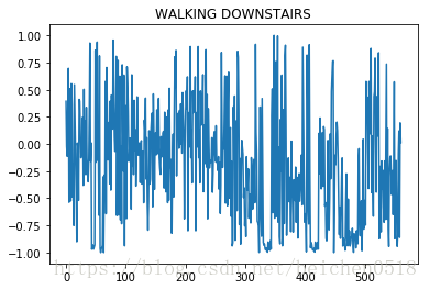
# 图形来表示动作
import matplotlib.pyplot as plt
plt.plot(X_train[1111])
# 加标题
plt.title(label[y_train[1111]])
输出
Text(0.5,1,’WALKING DOWNSTAIRS’)
# 进行数据训练,机器的学习
knn = KNeighborsClassifier(n_neighbors=15)
knn.fit(X_train, y_train)
输出
KNeighborsClassifier(algorithm=’auto’, leaf_size=30, metric=’minkowski’,
metric_params=None, n_jobs=1, n_neighbors=15, p=2,
weights=’uniform’)
# 开始进行预测
y_ = knn.predict(X_test)
y_
输出
array([5, 5, 5, …, 2, 2, 1], dtype=int64)
# 目标值
y_test
输出
array([5, 5, 5, …, 2, 2, 2], dtype=int64)
# 计算打分
knn.score(X_test, y_test)
输出
0.9043094672548354
# 人的动作对于机器来说就是频率,只要是频率都可以画图
# 将y_预测的数据对比y_test, 将这个答案作为标题
# argwhere(y_test == 1)
np.argwhere(y_test == 1).reshape(-1)
输出
array([ 79, 80, 81, 82, 83, 84, 85, 86, 87, 88, 89,
90, 91, 92, 93, 94, 95, 96, 97, 98, 99, 100,
101, 102, 103, 104, 105, 106, 107, 108, 227, 228, 229,
230, 231, 232, 233, 234, 235, 236, 237, 238, 239, 240,
241, 242, 243, 244, 245, 246, 247, 248, 249, 250, 251,
252, 253, 254, 255, 384, 385, 386, 387, 388, 389, 390,
391, 392, 393, 394, 395, 396, 397, 398, 399, 400, 401,
402, 403, 404, 405, 406, 407, 408, 409, 410, 411, 412,
413, 414, 544, 545, 546, 547, 548, 549, 550, 551, 552,
553, 554, 555, 556, 557, 558, 559, 560, 561, 562, 563,
564, 565, 566, 567, 568, 569, 570, 571, 572, 690, 691,
692, 693, 694, 695, 696, 697, 698, 699, 700, 701, 702,
703, 704, 705, 706, 707, 708, 709, 710, 711, 712, 713,
714, 715, 837, 838, 839, 840, 841, 842, 843, 844, 845,
846, 847, 848, 849, 850, 851, 852, 853, 854, 855, 856,
857, 858, 859, 860, 861, 862, 985, 986, 987, 988, 989,
990, 991, 992, 993, 994, 995, 996, 997, 998, 999, 1000,
1001, 1002, 1003, 1004, 1005, 1006, 1007, 1008, 1009, 1010, 1011,
1132, 1133, 1134, 1135, 1136, 1137, 1138, 1139, 1140, 1141, 1142,
1143, 1144, 1145, 1146, 1147, 1148, 1149, 1150, 1151, 1152, 1153,
1154, 1155, 1156, 1157, 1283, 1284, 1285, 1286, 1287, 1288, 1289,
1290, 1291, 1292, 1293, 1294, 1295, 1296, 1297, 1298, 1299, 1300,
1301, 1302, 1303, 1304, 1305, 1306, 1307, 1308, 1309, 1452, 1453,
1454, 1455, 1456, 1457, 1458, 1459, 1460, 1461, 1462, 1463, 1464,
1465, 1466, 1467, 1468, 1469, 1470, 1471, 1472, 1473, 1474, 1605,
1606, 1607, 1608, 1609, 1610, 1611, 1612, 1613, 1614, 1615, 1616,
1617, 1618, 1619, 1620, 1621, 1622, 1623, 1624, 1625, 1626, 1627,
1628, 1629, 1630, 1631, 1632, 1633, 1634, 1777, 1778, 1779, 1780,
1781, 1782, 1783, 1784, 1785, 1786, 1787, 1788, 1789, 1790, 1791,
1792, 1793, 1794, 1795, 1796, 1797, 1798, 1799, 1800, 1801, 1802,
1803, 1950, 1951, 1952, 1953, 1954, 1955, 1956, 1957, 1958, 1959,
1960, 1961, 1962, 1963, 1964, 1965, 1966, 1967, 1968, 1969, 1970,
1971, 1972, 1973, 1974, 1975, 1976, 1977, 1978, 2129, 2130, 2131,
2132, 2133, 2134, 2135, 2136, 2137, 2138, 2139, 2140, 2141, 2142,
2143, 2144, 2145, 2146, 2147, 2148, 2149, 2150, 2151, 2152, 2153,
2154, 2155, 2317, 2318, 2319, 2320, 2321, 2322, 2323, 2324, 2325,
2326, 2327, 2328, 2329, 2330, 2331, 2332, 2333, 2334, 2335, 2336,
2337, 2338, 2339, 2340, 2341, 2342, 2343, 2494, 2495, 2496, 2497,
2498, 2499, 2500, 2501, 2502, 2503, 2504, 2505, 2506, 2507, 2508,
2509, 2510, 2511, 2512, 2513, 2514, 2515, 2516, 2517, 2669, 2670,
2671, 2672, 2673, 2674, 2675, 2676, 2677, 2678, 2679, 2680, 2681,
2682, 2683, 2684, 2685, 2686, 2687, 2688, 2689, 2690, 2691, 2692,
2693, 2694, 2695, 2696, 2859, 2860, 2861, 2862, 2863, 2864, 2865,
2866, 2867, 2868, 2869, 2870, 2871, 2872, 2873, 2874, 2875, 2876,
2877, 2878, 2879, 2880, 2881, 2882, 2883, 2884, 2885, 2886, 2887,
2888], dtype=int64)
# 用循环来取值
plt.figure(figsize=(2*6, 3*5))
for i in range(6):
    # subplot第三个编号不能为0
    axes = plt.subplot(3, 2, i+1)
    np_index = np.argwhere(y_test == i + 1).reshape(-1)
    # 每个动作只取一个样本
    index = np_index[np.random.randint(0, np_index.size, size=1)[0]]

    axes.plot(X_test[index])
    # 给每张图片添加2个标题,分别是真实的答案,预测答案,但是只能用一个title,h换行、n
    axes.set_title('True:%s\n Predict:%s'%(label[y_test[index]], label[y_[index]]))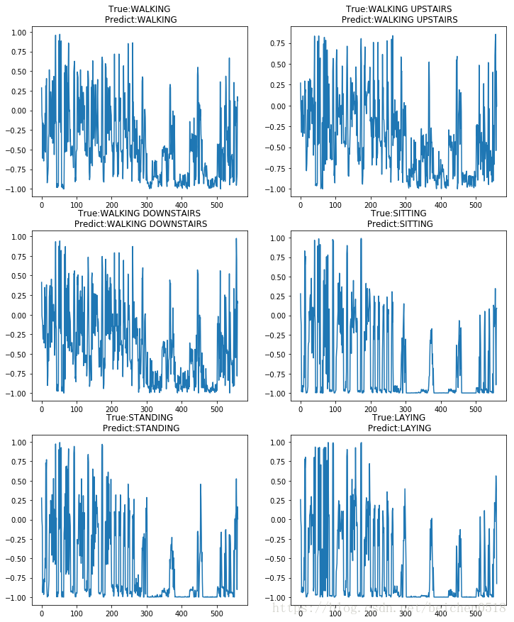
手写数字识别
#导入包
import numpy as np
import matplotlib.pyplot as plt
#引入机器学习
from sklearn.neighbors import KNeighborsClassifier
from sklearn.model_selection import train_test_split
#黑白图片
#2维的
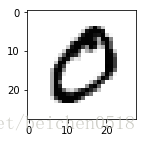
zero = plt.imread('./knn_num_data/0/0_1.bmp')
zero.shape输出
(28, 28)
plt.figure(figsize=(2,2))
plt.imshow(zero,cmap='gray')
<matplotlib.image.AxesImage at 0xada0828>
#怎么读取图片?
#用循环
#这是我们手动拼接的公用路径
path = './knn_num_data/%d/%d_%d.bmp'
data = []
target = []
#有10个目录
for i in range(10):
#下个循环500次,每个目录有500张图片
for j in range(500):
im_data = plt.imread(path%(i,i,j+1))
data.append(im_data)
target.append(i)data = np.array(data)
data输出
array([[[255, 255, 255, …, 255, 255, 255],
[255, 255, 255, …, 255, 255, 255],
[255, 255, 255, …, 255, 255, 255],
…,
[255, 255, 255, …, 255, 255, 255],
[255, 255, 255, …, 255, 255, 255],
[255, 255, 255, …, 255, 255, 255]],[[255, 255, 255, ..., 255, 255, 255], [255, 255, 255, ..., 255, 255, 255], [255, 255, 255, ..., 255, 255, 255], ..., [255, 255, 255, ..., 255, 255, 255], [255, 255, 255, ..., 255, 255, 255], [255, 255, 255, ..., 255, 255, 255]], [[255, 255, 255, ..., 255, 255, 255], [255, 255, 255, ..., 255, 255, 255], [255, 255, 255, ..., 255, 255, 255], ..., [255, 255, 255, ..., 255, 255, 255], [255, 255, 255, ..., 255, 255, 255], [255, 255, 255, ..., 255, 255, 255]], ..., [[255, 255, 255, ..., 255, 255, 255], [255, 255, 255, ..., 255, 255, 255], [255, 255, 255, ..., 255, 255, 255], ..., [255, 255, 255, ..., 255, 255, 255], [255, 255, 255, ..., 255, 255, 255], [255, 255, 255, ..., 255, 255, 255]], [[255, 255, 255, ..., 255, 255, 255], [255, 255, 255, ..., 255, 255, 255], [255, 255, 255, ..., 255, 255, 255], ..., [255, 255, 255, ..., 255, 255, 255], [255, 255, 255, ..., 255, 255, 255], [255, 255, 255, ..., 255, 255, 255]], [[255, 255, 255, ..., 255, 255, 255], [255, 255, 255, ..., 255, 255, 255], [255, 255, 255, ..., 255, 255, 255], ..., [255, 255, 255, ..., 255, 255, 255], [255, 255, 255, ..., 255, 255, 255], [255, 255, 255, ..., 255, 255, 255]]], dtype=uint8)
target = np.array(target)
target
输出
array([0, 0, 0, …, 9, 9, 9])
display(data.shape,target.size)- 输出
(5000, 28, 28)
5000
#现在的data是一个三维的,但是训练和预测数据只能是二维的?
data = data.reshape(5000,-1)
data.shape
输出
(5000, 784)
#要不要分开数据?
X_train,X_test,y_train,y_test=train_test_split(data,target,test_size=0.01)
#进行实例化
knn = KNeighborsClassifier(n_neighbors=5)#训练
knn.fit(X_train,y_train)输出
KNeighborsClassifier(algorithm=’auto’, leaf_size=30, metric=’minkowski’,
metric_params=None, n_jobs=1, n_neighbors=5, p=2,
weights=’uniform’)
#预测
y_ = knn.predict(X_test)
y_
输出
array([0, 2, 1, 3, 9, 8, 0, 4, 7, 5, 0, 8, 9, 3, 3, 2, 5, 5, 9, 8, 6, 9,
0, 0, 9, 0, 0, 3, 8, 0, 3, 0, 4, 3, 5, 7, 0, 3, 0, 9, 8, 7, 9, 6,
1, 5, 0, 3, 2, 2])
y_test输出
array([0, 2, 8, 3, 9, 8, 0, 4, 7, 5, 0, 8, 9, 5, 3, 2, 5, 5, 9, 8, 6, 9,
0, 0, 9, 0, 0, 3, 8, 0, 3, 0, 4, 3, 5, 3, 0, 3, 0, 9, 8, 7, 9, 6,
5, 5, 0, 3, 2, 2])
#得分
knn.score(X_test,y_test)
输出
0.92
画图
我们预测了50个手写数字,将这50个数字的图片给展示出来,将真实的目标值和预测的值作为标题
y_test[11]输出
8
##### 循环
plt.figure(figsize=(5*2,10*3))
for i in range(50):
    axes = plt.subplot(10,5,i+1)
    #X_test 784
    axes.imshow(X_test[i].reshape(28,28))
    #给标题
    t = y_test[i]
    p = y_[i]
    #设置标题
    axes.set_title('True:%s\nPredict:%s'%(t,p))
    axes.axis('off')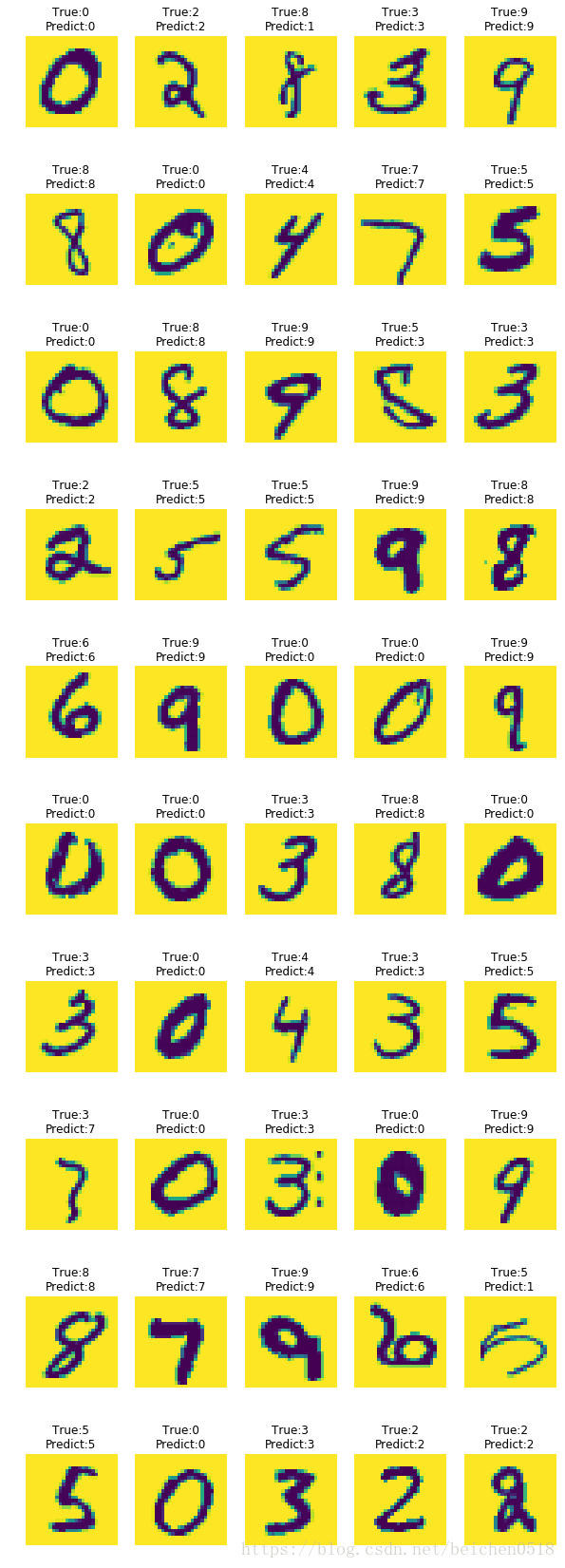
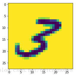
plt.imshow(X_test[4].reshape(28,28))<matplotlib.image.AxesImage at 0xb728a90>
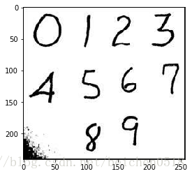
#读取网上的图片
num = plt.imread('./num_.jpg')
plt.imshow(num)
<matplotlib.image.AxesImage at 0xc2e2a90>
z = num[3:65,3:65]
plt.imshow(z)
<matplotlib.image.AxesImage at 0xc441f98>
z.shape- 输出
(62, 62, 3)
#降维
z = z.mean(axis=-1)
z.shape
输出
(62, 62)
#(28,28)
import cv2
#ndimage.zoom()
#cv2.resize()
z = cv2.resize(z,(28,28))
z.shape
输出
(28, 28)
#二维
x_test = np.array([z.reshape(-1)])knn.predict(x_test)- 输出
array([0])
换脸
import os, math
import cv2
from PIL import Image, ImageDraw
import matplotlib.pyplot as plt
# 1.将图片引入
sanpang = cv2.imread('./jinzhengen.png')
sanpang.shape输出
(273, 411, 3)
guobin = cv2.imread('./guobin.jpg')
guobin.shape
输出
(405, 259, 3)
# 加载面部识别的算法
face_detect = cv2.CascadeClassifier('./haarcascade_frontalface_default.xml')
sanpang_face = face_detect.detectMultiScale(sanpang)
guobin_face = face_detect.detectMultiScale(guobin)
display(sanpang_face, guobin_face)- 输出
array([[182, 62, 61, 61]], dtype=int32)
array([[ 32, 82, 164, 164]], dtype=int32)
# sanpang 的脸替换得到guobin的脸上
# 将三胖的脸切圆
# 先要获取到脸部的图片
for x, y, w, h in sanpang_face:
    sface = sanpang[y:y + h, x:x + w]
# guobin的脸
for x, y, w, h in guobin_face:
gface = guobin[y:y + h, x:x + w]plt.imshow(gface[:,:,::-1])<matplotlib.image.AxesImage at 0xc408e10>
sface = cv2.resize(sface, (164, 164))plt.imshow(sface[:,:,::-1])<matplotlib.image.AxesImage at 0xa202160>
# 把脸给它保存成图片
spath = './sface.png'
gpath = './gface.jpg'
new_path = './new_face.png'
cv2.imwrite(spath,sface)
cv2.imwrite(gpath,gface)输出
True
# a_path 代表要切圆的图片;b_path代表填补数据
def circle(a_path, b_path, new_path):
    # A alpha 代表透明度
    ima = Image.open(a_path).convert("RGBA")

    size = ima.size

    # 因为是要圆形,所以需要正方形的图片

    r2 = min(size[0], size[1])

    if size[0] != size[1]:
        # 抗锯齿
        ima = ima.resize((r2, r2), Image.ANTIALIAS)
    # 重新创建一个白色,画布
    imb = Image.new('RGBA', (r2, r2),(255,255,255,0))
    imc = Image.open(b_path).convert("RGBA")
    pima = ima.load()

    pimb = imb.load()

    pimc = imc.load()

    r = float(r2/2) #圆心横坐标

    for i in range(r2):

        for j in range(r2):

            lx = abs(i-r+0.5) #到圆心距离的横坐标

            ly = abs(j-r+0.5)#到圆心距离的纵坐标

            l  = pow(lx,2) + pow(ly,2)

            if l <= pow(r, 2):

                pimb[i,j] = pima[i,j]
            else:
                pimb[i,j] = pimc[i,j]

    imb.save(new_path)
circle(spath, gpath, new_path)# 原图是什么格式打开就是什么格式
trans = plt.imread(new_path)# 将图片转化为jpg打开,并且是rgb,而不是rgba
trans = cv2.imread(new_path)trans.shape输出
(164, 164, 3)
trans = trans[:,:,:-1]trans.shape输出
(164, 164, 3)
plt.imshow(trans)<matplotlib.image.AxesImage at 0xeb60f98>
for x, y, w, h in guobin_face:
guobin[y:y + h, x:x + w] = transplt.imshow(guobin[:,:,::-1])<matplotlib.image.AxesImage at 0x97c0da0>


 312
312

 被折叠的 条评论
为什么被折叠?
被折叠的 条评论
为什么被折叠?
 到【灌水乐园】发言


