数组属性和基本操作

数组属性和基本操作

np.arange(start=150,stop=0,step=-1)

• 将值倒过来

import numpy as np
#matplotlib画图的，也可以读取图片
import matplotlib.pyplot as plt
np.arange(150, 1, step=-1)

• 输出

  array([150, 149, 148, 147, 146, 145, 144, 143, 142, 141, 140, 139, 138,
  137, 136, 135, 134, 133, 132, 131, 130, 129, 128, 127, 126, 125,
  124, 123, 122, 121, 120, 119, 118, 117, 116, 115, 114, 113, 112,
  111, 110, 109, 108, 107, 106, 105, 104, 103, 102, 101, 100, 99,
  98, 97, 96, 95, 94, 93, 92, 91, 90, 89, 88, 87, 86,
  85, 84, 83, 82, 81, 80, 79, 78, 77, 76, 75, 74, 73,
  72, 71, 70, 69, 68, 67, 66, 65, 64, 63, 62, 61, 60,
  59, 58, 57, 56, 55, 54, 53, 52, 51, 50, 49, 48, 47,
  46, 45, 44, 43, 42, 41, 40, 39, 38, 37, 36, 35, 34,
  33, 32, 31, 30, 29, 28, 27, 26, 25, 24, 23, 22, 21,
  20, 19, 18, 17, 16, 15, 14, 13, 12, 11, 10, 9, 8,
  7, 6, 5, 4, 3, 2])

2.7 随机数组抽样

1.生成随机的整数型矩阵

np.random.randint(low=0,high=150,size=(5,4))

• low 表示的是最小值
• high 表示最大值
• size 是一个元祖类型

nd1 = np.random.randint(0, 155, size=(5, 4))

display(nd1.dtype)

• 输出

  dtype(‘int32’)

2. 标准的正态分布

np.random.randn(10,5)

• 输出
  没有固定的参数，每多加一个数字，代表多真假一个维度

nd2 = np.random.randn(10, 5)

nd2

• 输出

  array([[-7.17465685e-02, 8.97999644e-01, -1.01189107e+00,
  6.29572791e-01, -1.80740610e-01],
  [ 8.13237248e-01, 6.24399001e-01, -1.01024921e+00,
  -1.39402595e+00, 1.73300388e+00],
  [ 5.65812188e-01, -3.41566690e-01, 6.18996387e-01,
  -1.06630093e+00, 1.13662646e+00],
  [-1.90524270e-01, 4.14243506e-01, 2.99203707e-01,
  3.91685734e-02, -4.20081127e-01],
  [ 3.35201508e-01, 3.06824463e-02, 4.29531982e-01,
  2.65788533e-01, 9.24575924e-01],
  [ 6.00198193e-01, -8.21467127e-01, 1.10462529e+00,
  2.74473179e-01, 7.58630288e-01],
  [-5.74027894e-01, 2.38057571e-01, -1.34492521e+00,
  3.42149500e-01, -2.52783483e-01],
  [ 1.65575102e+00, -2.05932806e-01, -1.00664911e+00,
  -1.00871681e+00, -3.91605776e-01],
  [ 4.93294769e-01, 4.30644126e-02, 3.20789124e-01,
  1.00034941e+00, 1.00526627e-01],
  [ 1.47097903e-03, 2.69390841e-01, 3.96618545e-03,
  -2.89304322e-01, -3.07926840e-01]])

3.随机抽样

np.random.random(size=(456,730,3))

• size 表示形状

nd3 = np.random.random(size=(456, 730, 3))

# size 表示形状
# random随机生成0-1

plt.imshow(nd3)

<matplotlib.image.AxesImage at 0xed4e6d8>

nd3.dtype

• 输出

  dtype(‘float64’)

4.标准方差，代表数据的稳定性

np.random.normal(loc=170,scale=100,size=50)

normal也是一个正态分布的一个方法

生成一个一维数组
- location 是定位的的值
- scale 是波动值
- size 是数据长度

nd4 = np.random.normal(loc=200, scale=100, size=50)
nd4

• 输出

  array([-56.02232919, 153.45697237, 211.4699278 , 175.8184369 ,
  77.18195801, 316.30562106, 251.55919822, 249.03665012,
  214.84112035, 214.60311729, 60.12026691, 163.53327963,
  117.85773035, 169.87077409, 185.35857895, 336.48425501,
  168.53226238, 263.93486349, 285.09881005, 224.79650831,
  242.71883123, 233.49179984, 285.41369792, 126.59530067,
  194.95166998, 191.40061835, 288.26058067, 233.28608553,
  431.90448377, 162.51105433, 396.13946643, 104.43390237,
  74.23309279, 336.54800229, 92.09935907, 410.05980147,
  145.4054326 , 188.42084088, 272.32293993, 156.79765209,
  208.25501995, 252.51071293, 255.60679396, 194.88091883,
  203.67786615, 239.83429384, 292.21927586, 228.09728718,
  190.78466303, 258.07911366])

5.随机数

每一个数据，都是一个维度
rand 和 random 的区别：random 需要 size来描述形状，而rand只需要我们直接给值，通过值的数量来确定形状
np.random.rand(d1,d2,dn)

nd5 = np.random.rand(456, 730, 3)
nd5

• 输出

  array([[[0.48251924, 0.58360837, 0.50571184],
  [0.84015656, 0.64538107, 0.27610826],
  [0.91038242, 0.76890052, 0.21667493],
  …,
  [0.54192019, 0.5773379 , 0.97012533],
  [0.67118332, 0.482776 , 0.83270159],
  [0.05082725, 0.12324931, 0.43254904]],

     [[0.59763352, 0.82346195, 0.05238808],
      [0.88013475, 0.32720737, 0.66413674],
      [0.78427348, 0.7540094 , 0.31645346],
      ...,
      [0.486801  , 0.48158342, 0.79319007],
      [0.74409383, 0.33681167, 0.70245972],
      [0.8459772 , 0.30818404, 0.8559085 ]],
  
     [[0.95734985, 0.02237371, 0.19859254],
      [0.40804435, 0.46756388, 0.14389389],
      [0.84333377, 0.45708618, 0.93690335],
      ...,
      [0.95090075, 0.24181324, 0.60599297],
      [0.29234272, 0.08784666, 0.60669042],
      [0.38705636, 0.63969406, 0.39367339]],
  
     ...,
  
     [[0.60636193, 0.81418486, 0.55794838],
      [0.99319523, 0.89525226, 0.3027485 ],
      [0.11739645, 0.47303434, 0.77561122],
      ...,
      [0.15309203, 0.94459511, 0.97619881],
      [0.67865788, 0.0357113 , 0.33575641],
      [0.16167815, 0.04022808, 0.36632257]],
  
     [[0.67613125, 0.72950058, 0.45039344],
      [0.97297441, 0.04063427, 0.97781784],
      [0.30074768, 0.0473752 , 0.36833314],
      ...,
      [0.58241118, 0.71152678, 0.23845613],
      [0.76157266, 0.67666114, 0.94035192],
      [0.79084713, 0.89129279, 0.93983466]],
  
     [[0.24880475, 0.41904647, 0.4706133 ],
      [0.00705752, 0.67130627, 0.46979071],
      [0.1794662 , 0.34267615, 0.37759805],
      ...,
      [0.56038342, 0.82268221, 0.16605486],
      [0.58547802, 0.2627139 , 0.59724263],
      [0.25576816, 0.23193501, 0.1962647 ]]])
  

plt.imshow(nd5)

<matplotlib.image.AxesImage at 0xf56b320>

2.9 linspace 与 logspace

linspace是线性生成的，是全闭区间

回忆一下

nd6 = np.linspace(0, 150, num=151)
nd6

• 输出

  array([ 0., 1., 2., 3., 4., 5., 6., 7., 8., 9., 10.,
  11., 12., 13., 14., 15., 16., 17., 18., 19., 20., 21.,
  22., 23., 24., 25., 26., 27., 28., 29., 30., 31., 32.,
  33., 34., 35., 36., 37., 38., 39., 40., 41., 42., 43.,
  44., 45., 46., 47., 48., 49., 50., 51., 52., 53., 54.,
  55., 56., 57., 58., 59., 60., 61., 62., 63., 64., 65.,
  66., 67., 68., 69., 70., 71., 72., 73., 74., 75., 76.,
  77., 78., 79., 80., 81., 82., 83., 84., 85., 86., 87.,
  88., 89., 90., 91., 92., 93., 94., 95., 96., 97., 98.,
  99., 100., 101., 102., 103., 104., 105., 106., 107., 108., 109.,
  110., 111., 112., 113., 114., 115., 116., 117., 118., 119., 120.,
  121., 122., 123., 124., 125., 126., 127., 128., 129., 130., 131.,
  132., 133., 134., 135., 136., 137., 138., 139., 140., 141., 142.,
  143., 144., 145., 146., 147., 148., 149., 150.])

logspace是线性生成，并且以什么为底

start从几开始
stop 到数字结尾
num 生成多少个数
base 表示的是底数 默认以10为底

np.log10(100)
# 晚上自习的时候看一下 logn 的使用

• 输出

  2.0

nd7 = np.logspace(0, 150, num=151, base=np.e)
nd7

• 输出

  array([1.00000000e+00, 2.71828183e+00, 7.38905610e+00, 2.00855369e+01,
  5.45981500e+01, 1.48413159e+02, 4.03428793e+02, 1.09663316e+03,
  2.98095799e+03, 8.10308393e+03, 2.20264658e+04, 5.98741417e+04,
  1.62754791e+05, 4.42413392e+05, 1.20260428e+06, 3.26901737e+06,
  8.88611052e+06, 2.41549528e+07, 6.56599691e+07, 1.78482301e+08,
  4.85165195e+08, 1.31881573e+09, 3.58491285e+09, 9.74480345e+09,
  2.64891221e+10, 7.20048993e+10, 1.95729609e+11, 5.32048241e+11,
  1.44625706e+12, 3.93133430e+12, 1.06864746e+13, 2.90488497e+13,
  7.89629602e+13, 2.14643580e+14, 5.83461743e+14, 1.58601345e+15,
  4.31123155e+15, 1.17191424e+16, 3.18559318e+16, 8.65934004e+16,
  2.35385267e+17, 6.39843494e+17, 1.73927494e+18, 4.72783947e+18,
  1.28516001e+19, 3.49342711e+19, 9.49611942e+19, 2.58131289e+20,
  7.01673591e+20, 1.90734657e+21, 5.18470553e+21, 1.40934908e+22,
  3.83100800e+22, 1.04137594e+23, 2.83075330e+23, 7.69478527e+23,
  2.09165950e+24, 5.68572000e+24, 1.54553894e+25, 4.20121040e+25,
  1.14200739e+26, 3.10429794e+26, 8.43835667e+26, 2.29378316e+27,
  6.23514908e+27, 1.69488924e+28, 4.60718663e+28, 1.25236317e+29,
  3.40427605e+29, 9.25378173e+29, 2.51543867e+30, 6.83767123e+30,
  1.85867175e+31, 5.05239363e+31, 1.37338298e+32, 3.73324200e+32,
  1.01480039e+33, 2.75851345e+33, 7.49841700e+33, 2.03828107e+34,
  5.54062238e+34, 1.50609731e+35, 4.09399696e+35, 1.11286375e+36,
  3.02507732e+36, 8.22301271e+36, 2.23524660e+37, 6.07603023e+37,
  1.65163625e+38, 4.48961282e+38, 1.22040329e+39, 3.31740010e+39,
  9.01762841e+39, 2.45124554e+40, 6.66317622e+40, 1.81123908e+41,
  4.92345829e+41, 1.33833472e+42, 3.63797095e+42, 9.88903032e+42,
  2.68811714e+43, 7.30705998e+43, 1.98626484e+44, 5.39922761e+44,
  1.46766223e+45, 3.98951957e+45, 1.08446386e+46, 2.94787839e+46,
  8.01316426e+46, 2.17820388e+47, 5.92097203e+47, 1.60948707e+48,
  4.37503945e+48, 1.18925902e+49, 3.23274119e+49, 8.78750164e+49,
  2.38869060e+50, 6.49313426e+50, 1.76501689e+51, 4.79781333e+51,
  1.30418088e+52, 3.54513118e+52, 9.63666567e+52, 2.61951732e+53,
  7.12058633e+53, 1.93557604e+54, 5.26144118e+54, 1.43020800e+55,
  3.88770841e+55, 1.05678871e+56, 2.87264955e+56, 7.80867107e+56,
  2.12261687e+57, 5.76987086e+57, 1.56841351e+58, 4.26338995e+58,
  1.15890954e+59, 3.15024275e+59, 8.56324762e+59, 2.32773204e+60,
  6.32743171e+60, 1.71997426e+61, 4.67537478e+61, 1.27089863e+62,
  3.45466066e+62, 9.39074129e+62, 2.55266814e+63, 6.93887142e+63,
  1.88618081e+64, 5.12717102e+64, 1.39370958e+65])

np.logspace(0, 150, num=151, base=np.pi)

• 输出

  array([1.00000000e+00, 3.14159265e+00, 9.86960440e+00, 3.10062767e+01,
  9.74090910e+01, 3.06019685e+02, 9.61389194e+02, 3.02029323e+03,
  9.48853102e+03, 2.98090993e+04, 9.36480475e+04, 2.94204018e+05,
  9.24269182e+05, 2.90367727e+06, 9.12217118e+06, 2.86581460e+07,
  9.00322208e+07, 2.82844564e+08, 8.88582403e+08, 2.79156395e+09,
  8.76995680e+09, 2.75516318e+10, 8.65560042e+10, 2.71923707e+11,
  8.54273520e+11, 2.68377941e+12, 8.43134169e+12, 2.64878411e+13,
  8.32140071e+13, 2.61424513e+14, 8.21289330e+14, 2.58015653e+15,
  8.10580079e+15, 2.54651242e+16, 8.00010472e+16, 2.51330702e+17,
  7.89578687e+17, 2.48053460e+18, 7.79282928e+18, 2.44818952e+19,
  7.69121422e+19, 2.41626621e+20, 7.59092417e+20, 2.38475916e+21,
  7.49194186e+21, 2.35366295e+22, 7.39425024e+22, 2.32297222e+23,
  7.29783247e+23, 2.29268169e+24, 7.20267194e+24, 2.26278613e+25,
  7.10875227e+25, 2.23328039e+26, 7.01605727e+26, 2.20415940e+27,
  6.92457097e+27, 2.17541813e+28, 6.83427761e+28, 2.14705163e+29,
  6.74516164e+29, 2.11905503e+30, 6.65720770e+30, 2.09142348e+31,
  6.57040064e+31, 2.06415224e+32, 6.48472551e+32, 2.03723660e+33,
  6.40016755e+33, 2.01067193e+34, 6.31671218e+34, 1.98445366e+35,
  6.23434503e+35, 1.95857725e+36, 6.15305191e+36, 1.93303827e+37,
  6.07281883e+37, 1.90783230e+38, 5.99363194e+38, 1.88295501e+39,
  5.91547762e+39, 1.85840210e+40, 5.83834239e+40, 1.83416936e+41,
  5.76221298e+41, 1.81025260e+42, 5.68707626e+42, 1.78664770e+43,
  5.61291929e+43, 1.76335060e+44, 5.53972929e+44, 1.74035728e+45,
  5.46749366e+45, 1.71766379e+46, 5.39619995e+46, 1.69526621e+47,
  5.32583587e+47, 1.67316069e+48, 5.25638932e+48, 1.65134341e+49,
  5.18784831e+49, 1.62981062e+50, 5.12020106e+50, 1.60855860e+51,
  5.05343589e+51, 1.58758371e+52, 4.98754131e+52, 1.56688231e+53,
  4.92250596e+53, 1.54645086e+54, 4.85831865e+54, 1.52628582e+55,
  4.79496832e+55, 1.50638372e+56, 4.73244404e+56, 1.48674114e+57,
  4.67073505e+57, 1.46735469e+58, 4.60983072e+58, 1.44822103e+59,
  4.54972056e+59, 1.42933687e+60, 4.49039420e+60, 1.41069894e+61,
  4.43184144e+61, 1.39230405e+62, 4.37405218e+62, 1.37414902e+63,
  4.31701646e+63, 1.35623072e+64, 4.26072447e+64, 1.33854607e+65,
  4.20516650e+65, 1.32109202e+66, 4.15033298e+66, 1.30386556e+67,
  4.09621446e+67, 1.28686373e+68, 4.04280163e+68, 1.27008359e+69,
  3.99008527e+69, 1.25352226e+70, 3.93805632e+70, 1.23717688e+71,
  3.88670580e+71, 1.22104464e+72, 3.83602486e+72, 1.20512275e+73,
  3.78600479e+73, 1.18940848e+74, 3.73663695e+74])

2.11 diag

np.diag构建对角矩阵构建对角矩阵 np.diag(v,k=0)参数为列表即可

• v可以是一维或二维的矩阵
• k<0表示斜线在矩阵的下方
• k>0表示斜线在矩阵的上方

# 满秩矩阵
np.diag([1,2,3])

• 输出

  array([[1, 0, 0],
  [0, 2, 0],
  [0, 0, 3]])

2.12 文件 I/O 创建数组

2.12.1CSV

csv,dat是一种常用的数据格式化文件类型，为了从中读取数据，我们使用

numpy.genfromtxt()

#使用 `numpy.savetxt` 我们可以将 Numpy 数组保存到csv文件中:


M = np.random.rand(3,3) 
# 不管给什么样的后缀名，都会以TXT格式进行存储
np.savetxt("random-matrix.dat", M)

#函数。

# wget http://labfile.oss.aliyuncs.com/courses/348/stockholm_td_adj.dat  
import numpy as np  

data1=np.genfromtxt('./random-matrix.dat')
print(data1.shape) #(3.3)

data2=np.loadtxt('./random-matrix.dat')
print(data2.shape)  #(3.3)

data3=np.mafromtxt('./random-matrix.dat')
print(data3.shape)  #(3.3)

data4=np.ndfromtxt('./random-matrix.dat')
print(data4.shape) #(3.3)

data5=np.recfromtxt('./random-matrix.dat')
print(data5.shape) #(3.3)

(3, 3)
(3, 3)
(3, 3)
(3, 3)
(3, 3)

2.12.2 Numpy 原生文件类型

使用 numpy.save 与 numpy.load 保存和读取：

a=np.save("random-matrix-1.npy", M)  

np.load("random-matrix-1.npy")  

• 输出

  array([[0.72147967, 0.96083609, 0.08819009],
  [0.84168826, 0.92901361, 0.42336533],
  [0.31404165, 0.09710978, 0.66129327]])

3、ndarray 数组属性

ndim,shape,size

• ndim 数组的维度 （自己会计算）
• shape 形状（5,4，3）
• size 数组的总长度
• dtype 查看数据类型

[[[1, 2, 3],[1, 2, 3],[1, 2, 3]],[[1, 2, 3],[1, 2, 3],[1, 2, 3]],[[1, 2, 3],[1, 2, 3],[1, 2, 3]]]

nd8 = np.array([[[1, 2, 3],[1, 2, 3],[1, 2, 3]],[[1, 2, 3],[1, 2, 3],[1, 2, 3]],[[1, 2, 3],[1, 2, 3],[1, 2, 3]]])

nd8.shape

• 输出

  (3, 3, 3)

nd8.dtype

• 输出

  dtype(‘int32’)

nd8.ndim

• 输出

  3

nd8.size

• 输出

  27

3.1 ndarray.T

ndarray.T用于数组的转置，与 .transpose() 相同。

nd8

• 输出

  array([[[1, 2, 3],
  [1, 2, 3],
  [1, 2, 3]],

     [[1, 2, 3],
      [1, 2, 3],
      [1, 2, 3]],
  
     [[1, 2, 3],
      [1, 2, 3],
      [1, 2, 3]]])
  

nd8.T

• 输出

  array([[[1, 1, 1],
  [1, 1, 1],
  [1, 1, 1]],

     [[2, 2, 2],
      [2, 2, 2],
      [2, 2, 2]],
  
     [[3, 3, 3],
      [3, 3, 3],
      [3, 3, 3]]])
  

3.3ndarray.imag

ndarray.imag 用来输出数组包含元素的虚部。

imaginary number 虚数

nd8.imag

• 输出

  array([[[0, 0, 0],
  [0, 0, 0],
  [0, 0, 0]],

     [[0, 0, 0],
      [0, 0, 0],
      [0, 0, 0]],
  
     [[0, 0, 0],
      [0, 0, 0],
      [0, 0, 0]]])
  

3.4ndarray.real

ndarray.real用来输出数组包含元素的实部。

real number 实数

nd8.real

• 输出

  array([[[1, 2, 3],
  [1, 2, 3],
  [1, 2, 3]],

     [[1, 2, 3],
      [1, 2, 3],
      [1, 2, 3]],
  
     [[1, 2, 3],
      [1, 2, 3],
      [1, 2, 3]]])
  

3.5ndarray.itemsize

ndarray.itemsize输出一个数组元素的字节数。

nd8.dtype
# int32 --> 4个字节

• 输出

  dtype(‘int32’)

nd8.itemsize

4

3.6 ndarray.nbytes

ndarray.nbytes用来输出数组的元素总字节数。

nd8.size

• 输出

  27

# 27个基本元素，每个元素都是int32类型， 那么每个元素占用4个字节， 27*4

nd8.nbytes

• 输出

  108

3.7 ndarray.strides

ndarray.strides用来遍历数组时，输出每个维度中步进的字节数组。

# 第一个是最外层的数组，占用4个 字节，有三个第二维， 3 * 4， 第三维中有也有三个元素，3*（3*4）
nd8.strides[::-1]

• 输出
  (4, 12, 36)

4、Numpy 数组的基本操作

4.0.1索引

一维与列表完全一致

ndd = np.random.randint(0, 155, size=(5,4))
ndd

• 输出

  array([[ 88, 133, 137, 17],
  [ 96, 74, 115, 62],
  [ 2, 71, 57, 38],
  [126, 144, 2, 105],
  [ 69, 76, 115, 121]])

ndd[0, 0]
ndd[0, ::-1]

• 输出

  array([ 17, 137, 133, 88])

# png的图片的RGB取值范围0-1
# 彩色的图片是三维的，黑白图片是二维的
fish = plt.imread('./fish.png')

plt.imshow(fish)

<matplotlib.image.AxesImage at 0x104e86d8>

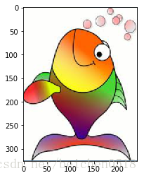
案例：颠倒图片

fish.shape

• 输出

  (326, 243, 3)

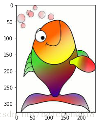
# 左右颠倒
fish1 = fish[:,::-1]
plt.imshow(fish1)

<matplotlib.image.AxesImage at 0x10ccabe0>

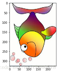
# 把fish1给上下颠倒
fish2 = fish1[::-1]
plt.imshow(fish2)

<matplotlib.image.AxesImage at 0x109306a0>

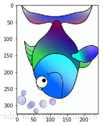
# RGB进行颠倒
fish3 = fish2[:,:,::-1]
plt.imshow(fish3)

<matplotlib.image.AxesImage at 0x107fb400>

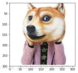
案例:把鱼头换成狗头

fish = plt.imread('./fish.png')
dog = plt.imread('dog.jpg')

fish.shape

• 输出

  (326, 243, 3)

plt.imshow(fish)

<matplotlib.image.AxesImage at 0x10b94c88>

dog.shape

• 输出

  (300, 313, 3)

plt.imshow(dog)

<matplotlib.image.AxesImage at 0x109cf5f8>

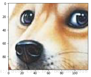
plt.imshow(fish[50:150, 70:190])

<matplotlib.image.AxesImage at 0x10a839b0>

plt.imshow(dog[50:150, 70:190])

<matplotlib.image.AxesImage at 0x10adae80>

# fish是png, # dog 是jpg
fish[50:180, 60:190] = dog[50:180, 60:190].astype(np.float32)/255

plt.imshow(fish)

<matplotlib.image.AxesImage at 0x11d3ecf8>

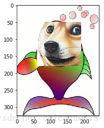
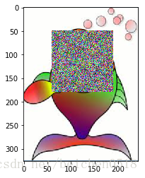
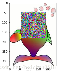
# 生成一张随机的图片，然后替换到鱼的头部
# randint(0-255, dtype=uint8)三维
# random再生成
nb9 = np.random.randint(0, 256, size=(130, 130, 3))
nb9 = nb9.astype(np.float32)
nb9.dtype
fish[50:180, 60:190] = nb9/255
plt.imshow(fish)

<matplotlib.image.AxesImage at 0x11d8bf98>

fish[50:150, 70:190] = np.random.random(size=(100, 120 ,3))
plt.imshow(fish)

<matplotlib.image.AxesImage at 0x11deb6d8>

4.1 重设形状

reshape 可以在不改变数组数据的同时，改变数组的形状。其中，numpy.reshape() 等效于 ndarray.reshape()。reshape方法非常简单：

nd1 = np.random.randint(0, 150, size=(5, 4))
nd1

• 输出

  array([[ 55, 59, 117, 33],
  [133, 41, 50, 134],
  [109, 99, 44, 96],
  [133, 34, 89, 33],
  [ 83, 1, 145, 13]])

# reshape(value) val 可以是单个值，这个值可以是list ,tuple
# 如果是多个值，这两值的乘积要等于原先形状的乘积
nd1.reshape((10, 2))

• 输出
  array([[ 55, 59],
  [117, 33],
  [133, 41],
  [ 50, 134],
  [109, 99],
  [ 44, 96],
  [133, 34],
  [ 89, 33],
  [ 83, 1],
  [145, 13]])

4.2.1 数组展开

ravel 的目的是将任意形状的数组扁平化，变为 1 维数组。ravel 方法如下：

# 将数组变为1维的，这种方式在数据中叫做扁平化
nd1.ravel()

• 输出

  array([ 55, 59, 117, 33, 133, 41, 50, 134, 109, 99, 44, 96, 133,
  34, 89, 33, 83, 1, 145, 13])

4. 2.2级联

1. np.concatenate() 级联需要注意的点：
2. 级联的参数是列表：一定要加中括号或小括号
3. 维度必须相同
4. 形状相符
5. 【重点】级联的方向默认是shape这个tuple的第一个值所代表的维度方向
6. 可通过axis参数改变级联的方向，默认为0, （0表示列相连,表示的X轴的事情，1表示行相连,Y轴的事情）

nd2 = np.random.randint(0, 150, size=(5, 4))
nd3 = np.random.randint(0, 150, size=(5, 4))
display(nd2, nd3)

• 输出
  array([[ 59, 110, 47, 76],
  [106, 121, 53, 126],
  [ 46, 8, 137, 124],
  [109, 88, 97, 99],
  [145, 48, 1, 6]])

  array([[ 4, 88, 136, 12],
  [ 62, 112, 75, 83],
  [ 98, 111, 144, 136],
  [146, 5, 44, 78],
  [126, 44, 30, 32]])

# axis 轴 默认值是0，表示的是对Y轴进行合并，或者说是垂直合并
# 垂直合并影响的是列，也就是说， 列的个数必须相等
np.concatenate([nd2, nd3]，axis=0)

• 输出

  array([[ 59, 110, 47, 76],
  [106, 121, 53, 126],
  [ 46, 8, 137, 124],
  [109, 88, 97, 99],
  [145, 48, 1, 6],
  [ 4, 88, 136, 12],
  [ 62, 112, 75, 83],
  [ 98, 111, 144, 136],
  [146, 5, 44, 78],
  [126, 44, 30, 32]])

# axis 轴 默认值是1，表示的是对X轴进行合并，或者说是水平合并
# 水平合并影响的是行，也就是说， 行的个数必须相等
np.concatenate([nd2, nd3], axis=1)

• 输出

  array([[ 59, 110, 47, 76, 4, 88, 136, 12],
  [106, 121, 53, 126, 62, 112, 75, 83],
  [ 46, 8, 137, 124, 98, 111, 144, 136],
  [109, 88, 97, 99, 146, 5, 44, 78],
  [145, 48, 1, 6, 126, 44, 30, 32]])

不同行数的数组合并

nd4 = np.random.randint(0, 150, size=(5, 4))
nd5 = np.random.randint(0, 150, size=(2, 4))
# 现在nd4和nd5需要怎么样级联
# 应该垂直级联 axis=0

不同的列数的数组合并

nd4 = np.random.randint(0, 150, size=(5, 4))
nd5 = np.random.randint(0, 150, size=(5, 3))
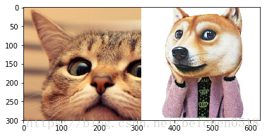
# 水平的级联

将猫和狗的图片合并

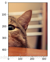
cat = plt.imread('cat.jpg')
dog = plt.imread('dog.jpg')

plt.imshow(cat)

<matplotlib.image.AxesImage at 0x88110b8>

cat.shape

• 输出

  (456, 730, 3)

dog.shape

• 输出
  (300, 313, 3)

plt.imshow(dog)

<matplotlib.image.AxesImage at 0x88a56d8>

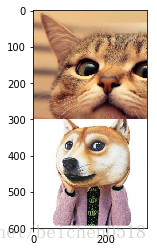
# 猫和狗怎么进行级联
# 把猫的图片切片
cat1 = cat[50:350, 100:413]
cat1.shape

• 输出

  (300, 313, 3)

# 垂直级联
cat_dog = np.concatenate((cat1, dog))
plt.imshow(cat_dog)

<matplotlib.image.AxesImage at 0x11e31ef0>

# 水平级联
cat_dog = np.concatenate((cat1, dog), axis=1)
plt.imshow(cat_dog)

<matplotlib.image.AxesImage at 0x131d25c0>

4.2.3 numpy.[hstack|vstack]

分别代表水平级联与垂直级联,填入的参数必须被小括号或中括号包裹

vertical垂直的 horizontal水平的 stack层积

这两个函数的值也是一个list或tuple

# cat_dog = np.concatenate((cat1, dog), axis=1)

dc = np.hstack((cat1, dog))
plt.imshow(dc)

<matplotlib.image.AxesImage at 0x1350a780>

cd = np.vstack((cat1, dog))
plt.imshow(cd)

<matplotlib.image.AxesImage at 0x13356cc0>

4.2.4分割数组

numpy.split(array,[index1,index2,…..]，axis)

axis默认值为0，表示垂直轴，如果值为1，表示水平的轴
注意：indices_or_sections ->[100, 200]列表中有两个值，第一个值代表0:100,第二个值代表100:200, 后面还有200: 会产生三个值，三个值需要三个变量来接收

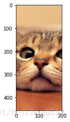
例题，将猫水平切成3份

cat1, cat2 ,cat3 = np.split(cat, [100, 200])
plt.imshow(cat1)
# show是用于图形显示的，不给值就是空的
plt.show()
plt.imshow(cat2)
plt.show()
plt.imshow(cat3)

<matplotlib.image.AxesImage at 0x13145710>

# 效果等同于split,不同于vsplit,它没有axis
cat1, cat2 ,cat3 = np.vsplit(cat, [100, 200])
plt.imshow(cat1)
# show是用于图形显示的，不给值就是空的
plt.show()
plt.imshow(cat2)
plt.show()
plt.imshow(cat3)

例题，将猫垂直切成3份

cat1, cat2 ,cat3 = np.split(cat, [200, 400],axis=1)
plt.imshow(cat1)
# show是用于图形显示的，不给值就是空的
plt.show()
plt.imshow(cat2)
plt.show()
plt.imshow(cat3)

<matplotlib.image.AxesImage at 0x134a4860>

cat1, cat2 ,cat3 = np.hsplit(cat, [200, 400])
plt.imshow(cat1)
# show是用于图形显示的，不给值就是空的
plt.show()
plt.imshow(cat2)
plt.show()
plt.imshow(cat3)

4.2.5副本

所有赋值运算不会为ndarray的任何元素创建副本。对赋值后的对象的操作也对原来的对象生效。

可使用ndarray.copy()函数创建副本

cat2 = cat.copy()
display(id(cat2),id(cat))

• 输出

  319763920
  141819616

4.2.6 ndarray的聚合函数

1. 求和np.sum

ndarray.sum(axis),axis不写则为所有的元素求和，为0表示列求和，1表示行求和

one = np.ones((5, 4))
one

• 输出

  array([[1., 1., 1., 1.],
  [1., 1., 1., 1.],
  [1., 1., 1., 1.],
  [1., 1., 1., 1.],
  [1., 1., 1., 1.]])

one.sum()

• 输出

  20.0

# axis = 0 我们认为是数组的第一层，1就是数组的第二层
# 不设置值的话就是全部求和
one.sum(axis=1)

• 输出

  array([4., 4., 4., 4., 4.])

求4维矩阵中最后两维的和

one_ = np.ones((3, 3, 3, 3 ))
# axis的值可以是一个元组，最后一维可以用-1来表示， -2可以用来表示倒数第二维
one_.sum(axis=(-1, -2))

• 输出

  array([[9., 9., 9.],
  [9., 9., 9.],
  [9., 9., 9.]])

2. 最大最小值：np.max/ np.min

cat.max(axis=1)

• 输出

  array([[242, 195, 140],
  [242, 195, 140],
  [241, 194, 140],
  …,
  [217, 134, 92],
  [217, 134, 92],
  [217, 134, 92]], dtype=uint8)

cat.min()

• 输出

  0

3.平均值:np.mean()

cat.mean()

• 输出

  132.22093747496595

cat.mean(axis=0)

• 输出

  array([[170.19298246, 116.40570175, 88.49122807],
  [170.52412281, 116.66666667, 88.75877193],
  [171.08991228, 117.36622807, 89.33114035],
  …,
  [105.55921053, 54.24122807, 47.26754386],
  [100.9122807 , 50.99122807, 44.29824561],
  [ 98.85087719, 50.05701754, 43.26973684]])

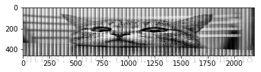
案例:将猫的图片黑白

cat2 = cat.reshape(456, 730*3)
cat2.shape

• 输出

  (456, 2190)

plt.imshow(cat2,cmap='gray')

<matplotlib.image.AxesImage at 0x8d1f438>

# 图片的第三维中的值怎么给它去掉
cat3 = cat.max(axis=2)
# cmap = 'color'黑白适用gray
plt.imshow(cat3, cmap='gray')

<matplotlib.image.AxesImage at 0x8c2e0f0>

cat3.shape

• 输出

  (456, 730)

cat4 = cat.min(axis=2)
plt.imshow(cat4, cmap='gray')

<matplotlib.image.AxesImage at 0x8d7add8>

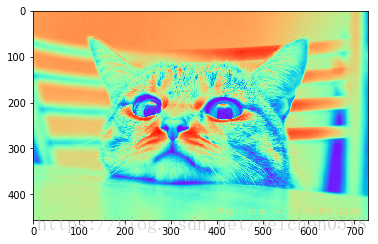
cat5 = cat.mean(axis=2)
plt.imshow(cat5, cmap='gray')

<matplotlib.image.AxesImage at 0x130c9b70>

cat6 = cat.mean(axis=2)
plt.imshow(cat5, cmap='rainbow')

<matplotlib.image.AxesImage at 0x8d6ab00>

4. 其他聚合操作

Function Name   NaN-safe Version    Description
np.sum  np.nansum   Compute sum of elements
np.prod np.nanprod  Compute product of elements
np.mean np.nanmean  Compute mean of elements
np.std  np.nanstd   Compute standard deviation
np.var  np.nanvar   Compute variance
np.min  np.nanmin   Find minimum value
np.max  np.nanmax   Find maximum value
np.argmin   np.nanargmin    Find index of minimum value 找到最小数的下标
np.argmax   np.nanargmax    Find index of maximum value
np.median   np.nanmedian    Compute median of elements
np.percentile   np.nanpercentile    Compute rank-based statistics of elements
np.any  N/A Evaluate whether any elements are true
np.all  N/A Evaluate whether all elements are true
np.power 幂运算
np.argwhere(nd1<0)

nd1 = np.random.randint(0, 255, size=(5,4))
nd1

array([[244,  20,  17, 194],
       [ 48, 241, 135, 135],
       [234, 246,  29, 160],
       [ 98, 166, 161,  44],
       [137,  10, 217,  94]])

# argmax最大值下标
cond = nd1.argmax()
nd2 = nd1.reshape(20)
nd2[cond]

• 输出

  246

# argwhere where相当于mysql中的where条件
index = np.argwhere(nd1 < 29)
index
nd1[index[:,0],index[:,1]]

• 输出

  array([20, 17, 10])

4.3 轴移动

moveaxis 可以将数组的轴移动到新的位置。其方法如下：

numpy.moveaxis(a, source, destination)  

其中：

• a：数组。
• source：要移动的轴的原始位置。

• destination：要移动的轴的目标位置。

  轴的移动就是维度的变化，以第一维度移动到第二维度为例，就是第一维度数据变成第二维度的数据，第二维度的数据变为第一维度，如果有3个维度，当第一维度移动到第三维度时，原来的第三维度变为第二维度，原来的第二维度变成第一维度

nd1 = np.array([[1,2,3], [1,2,3], [1,2,3]])
nd1

• 输出

  array([[1, 2, 3],
  [1, 2, 3],
  [1, 2, 3]])

np.moveaxis(nd1,0,1)

• 输出

  array([[1, 1, 1],
  [2, 2, 2],
  [3, 3, 3]])

4.4 轴交换

和 moveaxis 不同的是，swapaxes 可以用来交换数组的轴。其方法如下：

numpy.swapaxes(a, axis1, axis2) 

其中：

• a：数组。
• axes1：需要交换的轴 1 位置。
• axes2：需要与轴 1 交换位置的轴 1 位置。

与轴移动不同的是，轴的交换就是将两个维度的位置变化，其他维度不变，而轴移动，是移动位置到目标位置之间的维度都发生变化.

举个例子：

nd1 = np.random.randint(0, 100, size=(5, 4, 3))
nd1

• 输出
  array([[[ 3, 52, 42],
  [34, 92, 61],
  [99, 64, 42],
  [84, 63, 94]],

     [[70, 31, 75],
      [80, 13, 81],
      [ 6, 16, 71],
      [ 7, 99, 83]],
  
     [[19, 48, 55],
      [45, 53, 18],
      [12, 39, 39],
      [91, 66, 21]],
  
     [[40, 82, 91],
      [76, 54, 66],
      [21, 83, 47],
      [84,  5,  2]],
  
     [[ 8, 38, 97],
      [58, 76, 16],
      [41, 66, 78],
      [75, 17, 99]]])
  

np.swapaxes(nd1, 0, 2)

• 输出

  array([[[ 3, 70, 19, 40, 8],
  [34, 80, 45, 76, 58],
  [99, 6, 12, 21, 41],
  [84, 7, 91, 84, 75]],

     [[52, 31, 48, 82, 38],
      [92, 13, 53, 54, 76],
      [64, 16, 39, 83, 66],
      [63, 99, 66,  5, 17]],
  
     [[42, 75, 55, 91, 97],
      [61, 81, 18, 66, 16],
      [42, 71, 39, 47, 78],
      [94, 83, 21,  2, 99]]])
  

4.5 数组转置

transpose 类似于矩阵的转置，它可以将 2 维数组的水平轴和垂直交换。其方法如下：

numpy.transpose(a, axes=None)  

其中：

• a：数组。
• axis：该值默认为 none，表示转置。如果有值，那么则按照值替换轴。

nd1.transpose()
np.transpose(nd1)

• 输出

  array([[[ 3, 70, 19, 40, 8],
  [34, 80, 45, 76, 58],
  [99, 6, 12, 21, 41],
  [84, 7, 91, 84, 75]],

     [[52, 31, 48, 82, 38],
      [92, 13, 53, 54, 76],
      [64, 16, 39, 83, 66],
      [63, 99, 66,  5, 17]],
  
     [[42, 75, 55, 91, 97],
      [61, 81, 18, 66, 16],
      [42, 71, 39, 47, 78],
      [94, 83, 21,  2, 99]]])