Laplace方程求解

最新推荐文章于 2024-12-26 22:01:28 发布

转载最新推荐文章于 2024-12-26 22:01:28 发布 · 4.1k 阅读

文章标签：

#orthogonal #variables #mathematica #function #basic #types

算法同时被 3 个专栏收录

341 篇文章

订阅专栏

科学计算

326 篇文章

订阅专栏

图像处理

183 篇文章

订阅专栏

本文详细介绍了拉普拉斯方程的基本概念及其在不同边界条件下的求解方法，包括单一非齐次边界条件和四个非齐次边界条件的情况，并通过分离变量法等步骤给出具体解的形式。

摘要生成于 C知道，由 DeepSeek-R1 满血版支持，前往体验 >

Laplace Equation

From Wikiversity

Jump to: navigation, search

[hide]

1 Laplace Equation
- 1.1 Solution to Case with 1 Non-homogeneous Boundary Condition
- 1.2 Solution to Case with 4 Non-homogeneous Boundary Conditions

Laplace Equation[edit]

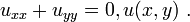
The Laplace equation is a basic PDE that arises in the heat and diffusion equations. The Laplace equation is defined as:

$\nabla^2 u = 0 \Rightarrow \frac{\partial^2 u}{\partial x_1^2} + \frac{\partial^2 u}{\partial x_2^2} + \frac{\partial^2 u}{\partial x_3^2} = 0 ~.$

Solution to Case with 1 Non-homogeneous Boundary Condition[edit]

In a condensed notation in (x,y,z) rectangular coordinates, the Laplace equation in two dimensions reduces to:

$u_{xx}+u_{yy} = 0, u(x,y) ~.$

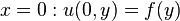
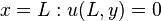
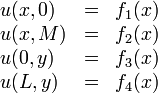
The solution to the case with 1 non-homogeneous boundary condition is the most basic solution type. For the purposes of this example, we consider that the following boundary conditions hold true for this equation:

$x=0: u(0,y)=f(y)$
$x=L: u(L,y)=0$
$y=0: u(x,0)=0$
$y=M: u(x,M)=0$

Step 1: Separate Variables[edit]

To solve this equation, we assume that the function $u(x,y)$ is comprised of two functions $\textstyle X(x)$ and 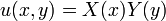$\textstyle Y(y)$ such that $\textstyle u(x,y)=X(x)Y(y)$ . Hence, $u_{xx}=X''(x)Y(y)$ and $u_{yy}=X(x)Y''(y) ~.$ Making the substitutions into the Laplace equation, we get:

$X''Y+XY''=0$

$\Rightarrow \frac{X''}{X} + \frac{Y''}{Y} = 0$

$\Rightarrow \frac{X''}{X} = -\frac{Y''}{Y} = \mu$

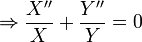
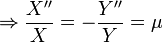
The $\mu$ is called a separation constant because the solution to the equation must yield a constant. Because of the separation constant, it yields two linear ODEs:

$X''-\mu X=0$
$Y''+\mu Y=0$

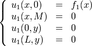
Step 2: Translate Boundary Conditions[edit]

Translating the boundary conditions allows us to divide the boundary conditions among the variables. This division yields:

$u(0,y)=X(0)Y(y)=f(x) \quad \forall y \in \lbrack 0,M \rbrack$
$u(L,y)=X(L)Y(y)=0 \quad \forall y \in \lbrack 0,M \rbrack \Rightarrow X(L)=0$
$u(x,0)=X(x)Y(y)=0 \quad \forall x \in \lbrack 0,L \rbrack \Rightarrow Y(0)=0$
$u(x,M)=X(x)Y(y)=0 \quad \forall x \in \lbrack 0,L \rbrack \Rightarrow Y(M)=0$

Step 3: Solve the Sturm-Liouville Problem[edit]

The last two boundary conditions are homogeneous boundary conditions for the function $Y(y)$ . Using the solution to the Sturm-Liouville problems (SLP), we can easily get a function for $Y(y)$ . The following is a fairly simple SLP:

$\begin{cases}Y''+\mu Y = 0 \\Y(0)=0 \\Y(M)=0 \end{cases}$

The solution to the SLP yields the following information:

$\mu = \frac{(n+1)^2\pi^2}{M^2},n=0,1,2,\cdots$
$Y_n(y)=\sin \frac{(n+1)\pi y}{M},n=0,1,2,\cdots$

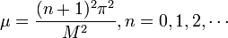
The solution we obtained is a family of solutions dependent on the value for n.

Step 4: Solve Remaining ODE[edit]

The remaining ODE that we have doesn't have a SLP solution to it because we only know one boundary condition for it. We have to use what we obtained from the SLP solution to help us solve this ODE. We obtained the following information from steps 1 and 2:

$\begin{cases}X''-\mu X = 0 \\X(L)=0 \end{cases}$

From analyzing the second order ODE, we obtain the characteristic equation $\textstyle m^2-\mu=0 \Rightarrow m^2=\mu \Rightarrow \mu = \pm \frac{(n+1)\pi}{M},n=0,1,2,\cdots ~.$ Out of the solution set that results from the exponentials, the only viable solution that arises is:

$X_n(x)=C_1 \cosh \frac{(n+1)\pi(x-L)}{M} + C_2 \sinh \frac{(n+1)\pi(x-L)}{M} ~.$

The substitution of (x-L) instead of x in the equation results only in a shift in the eigenspace, so it is valid and it helps us apply the boundary condition. Since 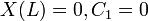$X(L)=0, C_1=0$ . For convenience, we choose $C_2=1~.$ The resulting equation is:

$X_n(x)=\sinh \frac{(n+1)\pi(x-L)}{M}, n=0,1,2,\cdots ~.$

Step 5: Combine Solutions[edit]

We obtained equations for our separate variable functions and now we can substitute into our assumption in step 1. The substitution yields:

$u_n(x,y)=\sinh \frac{(n+1)\pi(x-L)}{M} \sin \frac{(n+1)\pi y}{M}$

This function only satisfies the 3 homogeneous boundary conditions, however. To solve for the solution to the non-homogeneous boundary condition, we must consider that the complete solution consists of the following infinite series of terms:

$\begin{align}u(x,y) & :=\sum_{n=0}^\infty a_n u_n(x,y) \\& = \sum_{n=0}^\infty a_n \sinh \frac{(n+1)\pi(x-L)}{M} \sin \frac{(n+1)\pi y}{M}\end{align}$

At the non-homogeneous boundary condition:

$f(y)=u(0,y)=\sum_{n=0}^\infty \underbrace {a_n \sinh \frac{(n+1)\pi(0-L)}{M}}_{A_n} \sin \frac{(n+1)\pi y}{M}$

This is an orthogonal expansion of $f$ relative to the orthogonal basis of the sine function. The term $A_n$ is a Fourier coefficient which is defined as the inner product:

$A_n=\frac{\int\limits_{0}^{M} f(y)\sin(\frac{(n+1)\pi y}{M}) dy}{\int\limits_{0}^{M} \sin^2 \frac{(n+1)\pi y}{M}}=\frac{2}{M} \int\limits_{0}^{M} f(y)\sin(\frac{(n+1)\pi y}{M}) dy, n=0,1,2,\cdots$

Thus, the coefficient of the infinite series solution $a_n$ is:

$a_n=-\frac{2}{M\sinh\frac{(n+1)\pi L}{M}}\int\limits_{0}^{M} f(y)\sin\left(\frac{(n+1)\pi y}{M}\right) dy, n=0,1,2,\cdots~.$

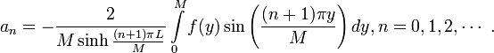
So, the entire general solution to the Laplace equation is:

$u(x,y)=\sum_{n=0}^\infty \left [ -\frac{2}{M\sinh\frac{(n+1)\pi L}{M}}\int\limits_{0}^{M} f(y)\sin\left(\frac{(n+1)\pi y}{M}\right) dy \right ] \sinh \frac{(n+1)\pi(x-L)}{M} \sin \frac{(n+1)\pi y}{M}~.$

This is the general solution for the specific set of boundary conditions we assumed at the beginning. Other boundary conditions will yield a different solution. You can see the solution graphically by entering in a partial sum (e.g. n starts at 0 and ends at 10) into a numerical solver like Mathematica or Maple.

Solution to Case with 4 Non-homogeneous Boundary Conditions[edit]

Because $\nabla^2$ is a linear operator, any solutions to the equation $\nabla^2u=0$ can be added together and the result will also be a solution to the equation. This is the superposition principle.

Because of superposition, we can solve the case where all four boundary conditions are non-homogeneous. To illustrate how this will work, let's take the boundary conditions:

$\begin{array}{lcl} u(x,0) & = & f_1(x) \\ u(x,M) & = & f_2(x) \\ u(0,y) & = & f_3(x) \\ u(L,y) & = & f_4(x)\end{array}$

We divide this problem into 4 sub-problems, each one containing one of the non-homogeneous boundary conditions and each one subject to the Laplace equation condition, $\frac{\partial^2}{\partial x^2}(u_n)+\frac{\partial^2}{\partial y^2}(u_n)=0~.$ We get the following boundary conditions for the 4 sub-problems:

$\left \{ \begin{array}{lcl} u_1(x,0) & = & f_1(x) \\ u_1(x,M) & = & 0 \\ u_1(0,y) & = & 0 \\ u_1(L,y) & = & 0\end{array} \right .$
$\left \{ \begin{array}{lcl} u_2(x,0) & = & 0 \\ u_2(x,M) & = & f_2(x) \\ u_2(0,y) & = & 0 \\ u_2(L,y) & = & 0\end{array} \right .$
$\left \{ \begin{array}{lcl} u_3(x,0) & = & 0 \\ u_3(x,M) & = & 0 \\ u_3(0,y) & = & f_3(x) \\ u_3(L,y) & = & 0\end{array} \right .$
$\left \{ \begin{array}{lcl} u_4(x,0) & = & 0 \\ u_4(x,M) & = & 0 \\ u_4(0,y) & = & 0 \\ u_4(L,y) & = & f_4(x)\end{array} \right .$

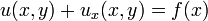In this case, we used all Dirichlet type boundary conditions, meaning that the boundary condition depends on the function value (e.g. $u(x,y)=f(x)$ ). If you are using any combination of Dirichlet, Neumann (e.g. $u_x(x,y)=f(x) ~.$ ), Robin (e.g. $u(x,y)+u_x(x,y)=f(x)$ ) types of boundary conditions, the types of the boundary conditions should be preserved in every sub-problem (e.g. if $u_x(L,y)=f(x)$ , then the boundary condition is $u_x(L,y)=0$ when the boundary condition is made homogeneous and $u_x(L,y)=f(x)$ when it is the non-homogeneous boundary condition in a sub-problem).

Using the superposition principle, the complete solution to the 4 non-homogeneous boundary condition case is constructed by adding up all the solutions from the 4 sub-problems. In equation form, $u(x,y)=u_1(x,y)+u_2(x,y)+u_3(x,y)+u_4(x,y)~.$ Each sub-problem can be solved using the method for the case with 1 non-homogeneous boundary condition as shown above.