


From: subce
Tips
整理一下关于绘图的基本设置,主要包括:
- 自定义legend
- 二维图tick的长度和粗细
- 孪生x轴、y轴
- 设置二维图边框粗细
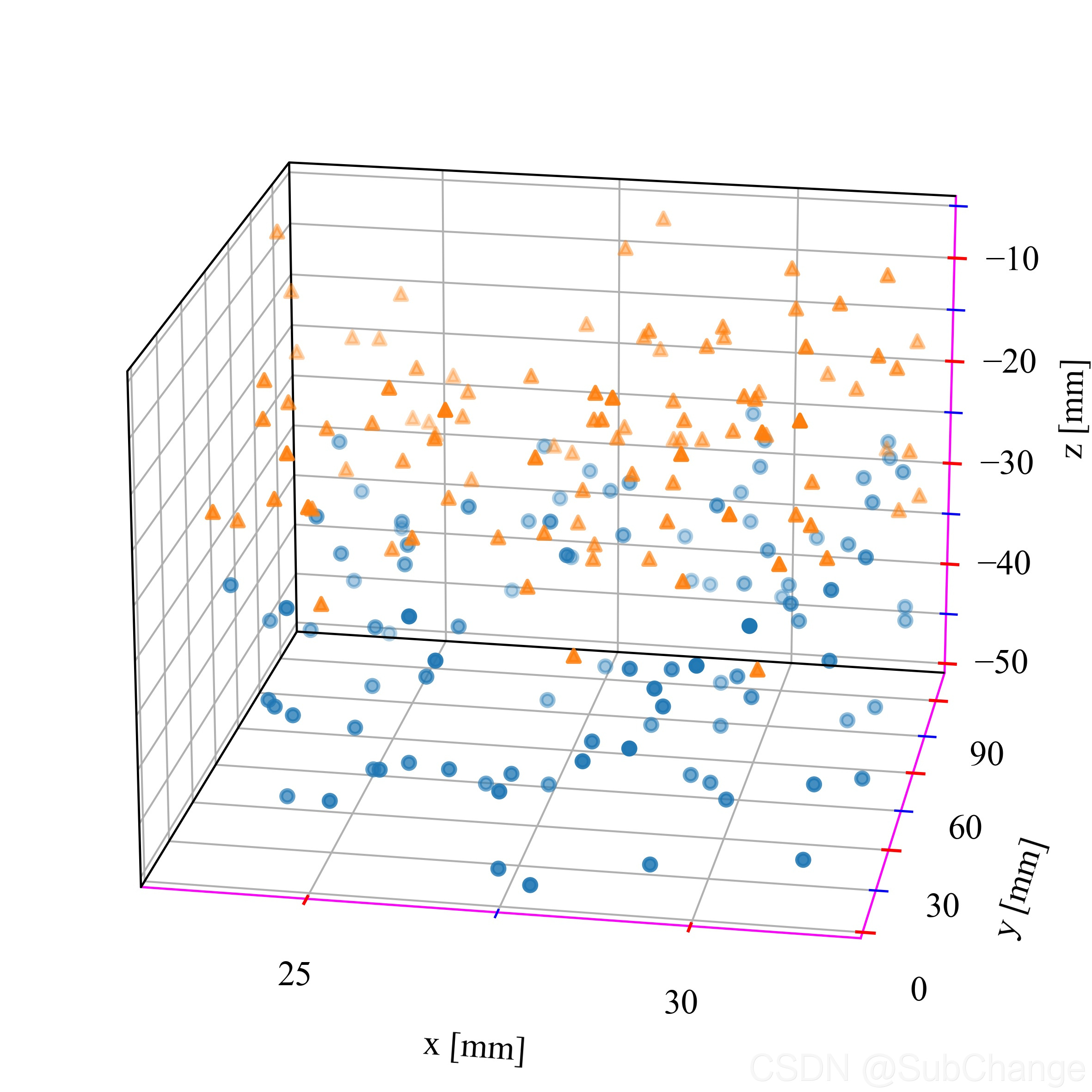
- 给三维图添加边框
- 设置三维图背景颜色为白色
- 三维图tick的长度和粗细
Legend
# 自定义legend
lenline1 = mlines.Line2D([], [], color='r', marker='s', linewidth=0.85,
                          markersize=5, label='Learning rate=0.0001')
lenline2 = mlines.Line2D([], [], color='g', marker='D', linewidth=0.85,
                          markersize=5, label='Learning rate=0.00001')
lenline3 = mlines.Line2D([], [], color='b', marker='^', linewidth=0.85,
                          markersize=5, label='Learning rate=0.001')

legend = ax.legend(handles=[lenline1,lenline2,lenline3], loc='lower right', bbox_to_anchor=(0.99, 0.01),ncol=1,frameon=True,fancybox=False,
                 facecolor='white',edgecolor='red')  # Add a legend.
2D
import numpy as np

import matplotlib as mpl
import matplotlib.pyplot as plt
from mpl_toolkits.mplot3d.axes3d import Axes3D

import matplotlib.font_manager as fm
from matplotlib.ticker import MultipleLocator,AutoMinorLocator


# 1pt = 0.35146mm = 0.035146cm
# 1inch = 2.54cm = 72.27pt
# 图表坐标轴线条粗细最佳为 0.2mm = [0.57pt]
# 线条粗细在0.1mm-0.4mm之间 >>> 0.3mm = [0.85pt]
# 原则上不超过14号字,尽量使用7-12号字,尽量少使用小于6号以下的字体
# 最多见的文字大小推荐使用7、8、9号字 >> [9pt]

# 图片大小 单位厘米
fw = 10/2.54
fh = 8/2.54

# 设置全局的字体
mpl.rcParams['font.family'] = 'serif'
mpl.rcParams['font.serif'] = 'Times New Roman'
mpl.rcParams['font.style'] = 'normal'
mpl.rcParams['font.variant'] = 'normal'
mpl.rcParams['font.weight'] = 'normal'
mpl.rcParams['font.stretch'] ='normal'
mpl.rcParams['font.size'] = 9

# 第一种方式设置字体
font0 = {'fontfamily': 'serif',
         'fontname': 'Times New Roman',
         'fontstyle': 'normal',
         'fontvariant': 'normal',
         'fontweight': 'normal',
         'fontstretch': 'normal',
         'fontsize': 9}

# 第二种方式设置字体
tick_font = fm.FontProperties(family='Times New Roman', style='normal', variant='normal', weight='normal',
                           stretch='normal', size=9)
x = np.linspace(0, 2, 100)

# 1pt = 0.35146mm = 0.035146cm
# 1inch = 2.54cm = 72.27pt

#plt.rcParams['xtick.direction'] = 'in'
#plt.rcParams['ytick.direction'] = 'in'
fig = plt.figure(figsize=(fw,fh))
# figsize=(8/2.54,6/2.54),dpi=72
ax = fig.add_subplot(111)  # Create a figure and an axes.

ax.plot(x, x, label='linear',linewidth=0.85)  # Plot some data on the axes.
ax.plot(x, x**2, label='quadratic',linewidth=0.85)  # Plot more data on the axes...
ax.plot(x, x**3, label='cubic',linewidth=0.85)  # ... and some more.

# 图形四周是否显示tick
ax.tick_params(bottom=True, top=True, left=True, right=True)
# 图形四周是否显示tick_label
ax.tick_params(labelbottom=True, labeltop=False, labelleft=True, labelright=False)

#ax.tick_params(which='both', width=2)
#ax.tick_params(which='major', length=7)
#ax.tick_params(which='minor', length=4, color='r')


# axis --> 坐标轴
# which --> 主要和次要tick ”both" "major" minor"
ax.tick_params(axis="both", which='both', direction="in") # length=16, width=2, color="turquoise"
ax.tick_params(axis="both", which='both', direction="in")


ax.xaxis.set_major_locator(MultipleLocator(base=0.5))
#ax.xaxis.set_minor_locator(MultipleLocator(base=0.1))
#ax.xaxis.set_minor_locator(AutoMinorLocator(n=5))

ax.yaxis.set_major_locator(MultipleLocator(base=1))
#ax.yaxis.set_minor_locator(AutoMinorLocator(n=2))

# 设置tick的长度和宽度
for xtl in  ax.get_xticklines():
    xtl.set_markersize(2) #length
    xtl.set_markeredgewidth(0.57) #width

for ytl in  ax.get_yticklines():
    ytl.set_markersize(2)
    ytl.set_markeredgewidth(0.57)

# 设置tick_label字体
for xtlabel in ax.get_xticklabels():
    xtlabel.set_fontproperties(tick_font)

for ytlabel in ax.get_yticklabels():
    ytlabel.set_fontproperties(tick_font)


#ax.set_xticks(np.linspace(0,2,5),minor=False)
#ax.set_xticks(np.linspace(0,2,21),minor=True)

#ax.set_yticks(np.linspace(0,9,10),minor=False)
#ax.set_yticks(np.linspace(0,9,19),minor=True)

#ax.minorticks_off()

# tick_label 为公式
#ticks = [-np.pi/2,np.pi/2.]
#labels = [r"$-\frac{\pi}{2}$",r"$\frac{\pi}{2}$"]
#ax.xaxis.set_minor_locator(ticker.FixedLocator(ticks))
#ax.xaxis.set_minor_formatter(ticker.FixedFormatter(labels))

# 设置图形变宽线宽度和颜色
bwith = 0.57
ax.spines['left'].set_color((0,0,0,1))
ax.spines['left'].set_linewidth(bwith)
ax.spines['right'].set_color((0,0,0,1))
ax.spines['right'].set_linewidth(bwith)
ax.spines['top'].set_color((0,0,0,1))
ax.spines['top'].set_linewidth(bwith)
ax.spines['bottom'].set_color((0,0,0,1))
ax.spines['bottom'].set_linewidth(bwith)

#ax.spines['left'].set_color('black')
#ax.spines['bottom'].set_linewidth(bwith)

# 设置图形坐标轴标签和标题字体
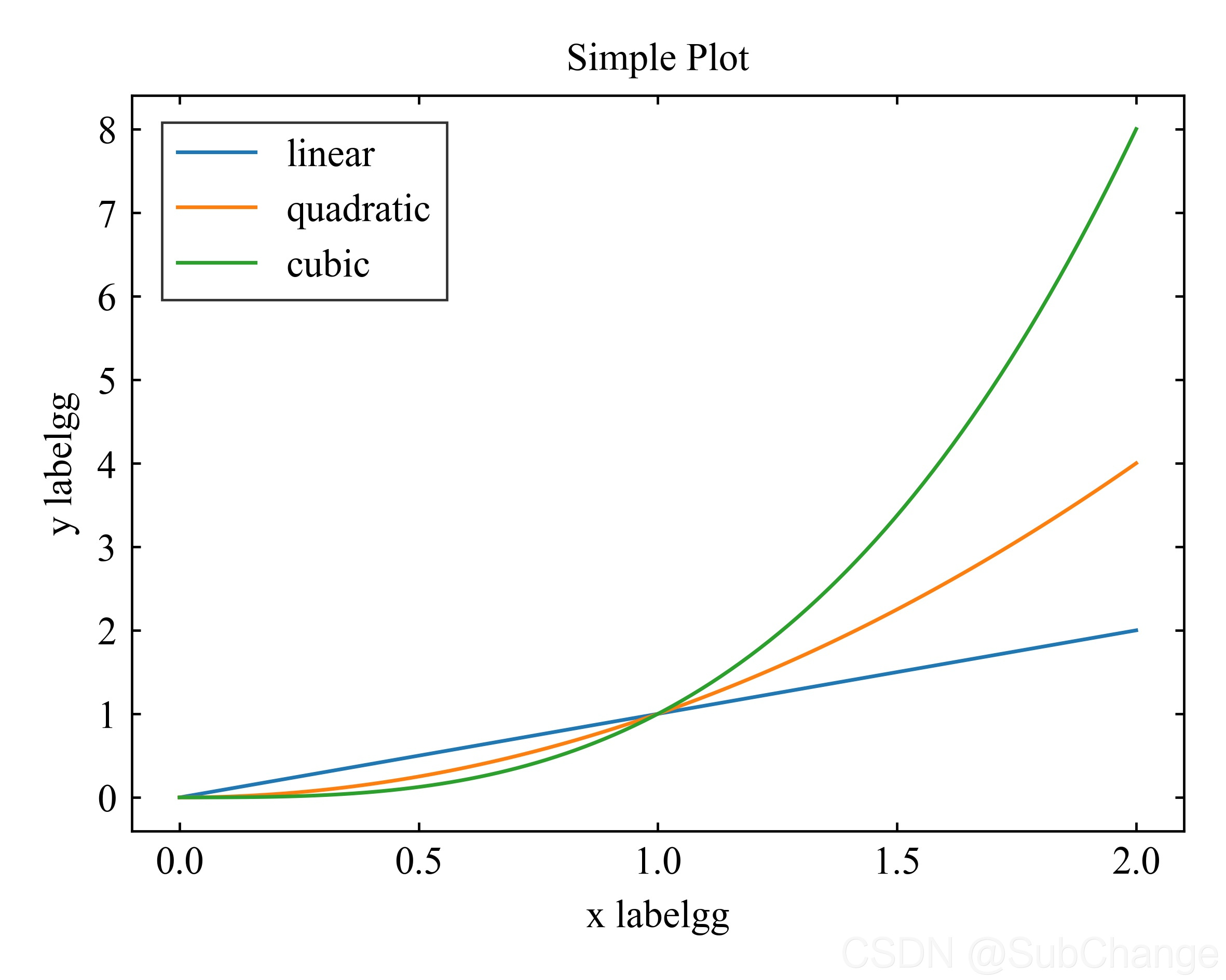
ax.set_xlabel('x labelgg',fontdict=font0)  # Add an x-label to the axes.
ax.set_ylabel('y labelgg',fontdict=font0)  # Add a y-label to the axes.
ax.set_title("Simple Plot",fontdict=font0)  # Add a title to the axes.

legend = ax.legend(loc='upper left', bbox_to_anchor=(0.01, 0.99),ncol=1,frameon=True,fancybox=False,
                 facecolor='white',edgecolor='red')  # Add a legend.
frame = legend.get_frame()
frame.set_linewidth(0.57) # 设置图例边框线宽
frame.set_edgecolor("black") # 设置图例边框颜色

plt.tight_layout()
plt.savefig('E:/Users/SubChange/Desktop/dd.tiff',dpi=600)
plt.show()
2D-twinxy
'''
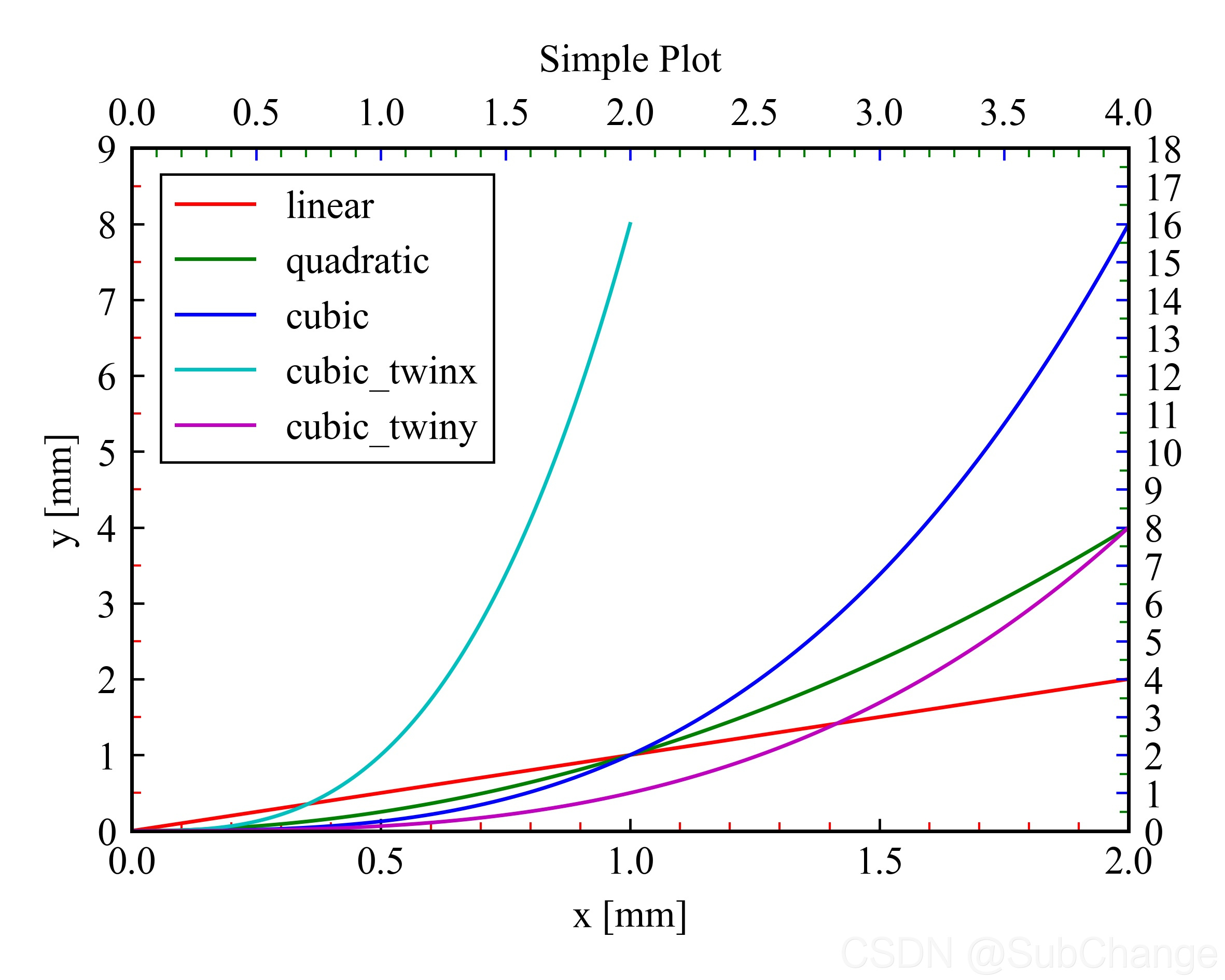
基本同上,注意两个y轴的设置
'''

import numpy as np

import matplotlib as mpl
import matplotlib.lines as mlines
import matplotlib.pyplot as plt
from mpl_toolkits.mplot3d.axes3d import Axes3D

import matplotlib.font_manager as fm
from matplotlib.ticker import MultipleLocator,AutoMinorLocator,NullLocator


# 1pt = 0.35146mm = 0.035146cm
# 1inch = 2.54cm = 72.27pt
# 图表坐标轴线条粗细最佳为 0.2mm = [0.57pt]
# 线条粗细在0.1mm-0.4mm之间 >>> 0.3mm = [0.85pt]
# 原则上不超过14号字,尽量使用7-12号字,尽量少使用小于6号以下的字体
# 最多见的文字大小推荐使用7、8号字 >> [8pt]

fw = 10/2.54
fh = 8/2.54

mpl.rcParams['font.family'] = 'serif'
mpl.rcParams['font.serif'] = 'Times New Roman'
mpl.rcParams['font.style'] = 'normal'
mpl.rcParams['font.variant'] = 'normal'
mpl.rcParams['font.weight'] = 'normal'
mpl.rcParams['font.stretch'] ='normal'
mpl.rcParams['font.size'] = 9

#mpl.rcParams['xtick.minor.size'] = 10
#mpl.rcParams['xtick.minor.width'] = 2

font0 = {'fontfamily': 'serif',
         'fontname': 'Times New Roman',
         'fontstyle': 'normal',
         'fontvariant': 'normal',
         'fontweight': 'normal',
         'fontstretch': 'normal',
         'fontsize': 9}

tick_font = fm.FontProperties(family='Times New Roman', style='normal', variant='normal', weight='normal',
                           stretch='normal', size=9)
x = np.linspace(0, 2, 100)

# 1pt = 0.35146mm = 0.035146cm
# 1inch = 2.54cm = 72.27pt

#plt.rcParams['xtick.direction'] = 'in'
#plt.rcParams['ytick.direction'] = 'in'
fig = plt.figure(figsize=(fw,fh))
# figsize=(8/2.54,6/2.54),dpi=72
ax = fig.add_subplot(111)  # Create a figure and an axes.

ax.plot(x, x, label='linear',linewidth=0.85,c='r')  # Plot some data on the axes.
ax.plot(x, x**2, label='quadratic',linewidth=0.85,c='g')  # Plot more data on the axes...
ax.plot(x, x**3, label='cubic',linewidth=0.85,c='b')  # ... and some more.


ax.set_xlim([0,2])
ax.set_ylim([0,9])
ax.tick_params(bottom=True, top=True, left=True, right=True)
ax.tick_params(labelbottom=True, labeltop=True, labelleft=True, labelright=True)

#ax.tick_params(which='both', width=2)
#ax.tick_params(which='major', length=7)
#ax.tick_params(which='minor', length=4, color='r')

ax.tick_params(axis="both", which='both', direction="in") # length=16, width=2, color="turquoise"

ax.tick_params(axis="both", which='minor', length=2.1, width=0.5, color="red") # length=16, width=2, color="turquoise"


ax.xaxis.set_major_locator(MultipleLocator(base=0.5))
#ax.xaxis.set_minor_locator(MultipleLocator(base=0.1))
ax.xaxis.set_minor_locator(AutoMinorLocator(n=5))

ax.yaxis.set_major_locator(MultipleLocator(base=1))
ax.yaxis.set_minor_locator(AutoMinorLocator(n=2))

for xtl in  ax.get_xticklines():
    xtl.set_markersize(2.85) #length
    xtl.set_markeredgewidth(0.57)

for ytl in  ax.get_yticklines():
    ytl.set_markersize(2.85)
    ytl.set_markeredgewidth(0.57)


for xtlabel in ax.get_xticklabels():
    xtlabel.set_fontproperties(tick_font)

for ytlabel in ax.get_yticklabels():
    ytlabel.set_fontproperties(tick_font)


#ax.set_xticks(np.linspace(0,2,5),minor=False)
#ax.set_xticks(np.linspace(0,2,21),minor=True)

#ax.set_yticks(np.linspace(0,9,10),minor=False)
#ax.set_yticks(np.linspace(0,9,19),minor=True)

#ax.minorticks_off()

#ticks = [-np.pi/2,np.pi/2.]
#labels = [r"$-\frac{\pi}{2}$",r"$\frac{\pi}{2}$"]
#ax.xaxis.set_minor_locator(ticker.FixedLocator(ticks))
#ax.xaxis.set_minor_formatter(ticker.FixedFormatter(labels))

bwith = 0.57
ax.spines['left'].set_color((0,0,0,1))
ax.spines['left'].set_linewidth(bwith)
#ax.spines['right'].set_color((0,0,0,1))
#ax.spines['right'].set_linewidth(bwith)
#ax.spines['top'].set_color((0,0,0,1))
#ax.spines['top'].set_linewidth(bwith)
ax.spines['bottom'].set_color((0,0,0,1))
ax.spines['bottom'].set_linewidth(bwith)

#ax.spines['left'].set_color('black')
#ax.spines['bottom'].set_linewidth(bwith)

# =====================================================
# 设置第二个y轴
axw = ax.twiny()
axw.set_xlim([0,2])
axw.tick_params(axis="x", which='both', direction="in", color='b')
axw.tick_params(axis="x", which='minor', length=2.1, width=0.5, color="green")
axw.xaxis.set_major_locator(MultipleLocator(base=0.5))
axw.xaxis.set_minor_locator(AutoMinorLocator(n=5))
for xwtl in  axw.get_xticklines():
    xwtl.set_markersize(2.85)
    xwtl.set_markeredgewidth(0.57)

axw.set_xlim([0,4])
axw.set_ylim([0,9])
axw.plot(x, x**3, label='cubic_twinx',linewidth=0.85,c='c')  # Plot more data on the axes...


# 设置第二个x轴
ayw = ax.twinx()
ayw.set_ylim([0,9])
ayw.tick_params(axis="y", which='both', direction="in", color='b')
ayw.tick_params(axis="y", which='minor', length=2.1, width=0.5, color="green")
ayw.yaxis.set_major_locator(MultipleLocator(base=1))
ayw.yaxis.set_minor_locator(AutoMinorLocator(n=2))
for ywtl in  ayw.get_yticklines():
    ywtl.set_markersize(2.85)
    ywtl.set_markeredgewidth(0.57)

ayw.set_xlim([0,2])
ayw.set_ylim([0,18])
ayw.plot(x, x**3, label='cubic_twiny',linewidth=0.85,c='m')  # ... and some more.


ax.set_xlabel('x [mm]',fontdict=font0)  # Add an x-label to the axes.
ax.set_ylabel('y [mm]',fontdict=font0)  # Add a y-label to the axes.
ax.set_title("Simple Plot",fontdict=font0)  # Add a title to the axes.


# 自定义legend
lenline1 = mlines.Line2D([], [], color='r', marker='', linewidth=0.85,
                          markersize=5, label='linear')
lenline2 = mlines.Line2D([], [], color='g', marker='', linewidth=0.85,
                          markersize=5, label='quadratic')
lenline3 = mlines.Line2D([], [], color='b', marker='', linewidth=0.85,
                          markersize=5, label='cubic')
lenline4 = mlines.Line2D([], [], color='c', marker='', linewidth=0.85,
                          markersize=5, label='cubic_twinx')
lenline5 = mlines.Line2D([], [], color='m', marker='', linewidth=0.85,
                          markersize=5, label='cubic_twiny')

legend = ax.legend(handles=[lenline1,lenline2,lenline3,lenline4,lenline5], loc='upper left', bbox_to_anchor=((0.01, 0.99)),ncol=1,frameon=True,fancybox=False,
                 facecolor='white',edgecolor='k',framealpha=1.0)  # Add a legend.
frame = legend.get_frame()
frame.set_linewidth(0.57)
frame.set_edgecolor("black")


plt.tight_layout()
plt.savefig('E:/Users/SubChange/Desktop/dd1.jpg',dpi=600)
plt.show()
3D
import numpy as np

import matplotlib as mpl
import matplotlib.pyplot as plt
from mpl_toolkits.mplot3d.axes3d import Axes3D
from mpl_toolkits.mplot3d import art3d

import matplotlib.font_manager as fm
from matplotlib.ticker import MultipleLocator,AutoMinorLocator,NullLocator


# 全局字体参数
mpl.rcParams['font.family'] = 'serif'
mpl.rcParams['font.serif'] = 'Times New Roman'
mpl.rcParams['font.style'] = 'normal'
mpl.rcParams['font.variant'] = 'normal'
mpl.rcParams['font.weight'] = 'normal'
mpl.rcParams['font.stretch'] ='normal'
mpl.rcParams['font.size'] = 9

#mpl.rcParams['xtick.minor.size'] = 10
#mpl.rcParams['xtick.minor.width'] = 2

# 字体1
font0 = {'fontfamily': 'serif',
         'fontname': 'Times New Roman',
         'fontstyle': 'normal',
         'fontvariant': 'normal',
         'fontweight': 'normal',
         'fontstretch': 'normal',
         'fontsize': 9}

# 字体2
tick_font = fm.FontProperties(family='Times New Roman', style='normal', variant='normal', weight='normal',
                           stretch='normal', size=9)


# Fixing random state for reproducibility
np.random.seed(19680801)


'''
因为matplotlib默认不会在3d图上添加边框,这里需要手动添加
'''
def add_borders(ax,edgecolor=(0,0,0,1),linewidth=0.57,scale=1.021):
    #ax.xaxis.pane.set_edgecolor(edgecolor)
    #ax.xaxis.pane.set_linewidth(linewidth)
    #ax.yaxis.pane.set_edgecolor(edgecolor)
    #ax.yaxis.pane.set_linewidth(linewidth)
    #ax.zaxis.pane.set_edgecolor(edgecolor)
    #ax.zaxis.pane.set_linewidth(linewidth)

    #ax.xaxis.pane.set_alpha(1)
    #ax.yaxis.pane.set_alpha(1)
    #ax.zaxis.pane.set_alpha(1)

    #ax.zaxis._axinfo['juggled'] = (1,2,0)
    xlims = ax.get_xlim3d()
    xoffset = (xlims[1] - xlims[0])*scale
    xlims = np.array([xlims[1] - xoffset, xlims[0] + xoffset])
    ylims = ax.get_ylim3d()
    yoffset = (ylims[1] - ylims[0])*scale
    ylims = np.array([ylims[1] - yoffset, ylims[0] + yoffset])
    zlims = ax.get_zlim3d()
    zoffset = (zlims[1] - zlims[0])*scale
    zlims = np.array([zlims[1] - zoffset, zlims[0] + zoffset])

    verts1 = np.array([[xlims[0], ylims[1], zlims[0]],
                       [xlims[0], ylims[0], zlims[0]],
                       [xlims[0], ylims[0], zlims[1]],
                       [xlims[0], ylims[1], zlims[1]]])

    verts2 = np.array([[xlims[1], ylims[1], zlims[0]],
                       [xlims[0], ylims[1], zlims[0]],
                       [xlims[0], ylims[1], zlims[1]],
                       [xlims[1], ylims[1], zlims[1]]])
    #i = np.array([xlims[0], ylims[0], zlims[0]])
    #f = np.array([xlims[0], ylims[0], zlims[1]])
    p = art3d.Line3DCollection([verts1,verts2],facecolor=(1,1,1,0),colors=edgecolor,linewidths=linewidth)
    ax.add_collection3d(p)
    return True


def randrange(n, vmin, vmax):
    """
    Helper function to make an array of random numbers having shape (n, )
    with each number distributed Uniform(vmin, vmax).
    """
    return (vmax - vmin)*np.random.rand(n) + vmin

# 图形大小 单位:厘米
fw = 10/2.54
fh = 10/2.54

fig = plt.figure(figsize=(fw,fh),facecolor=(1.0,1.0,1.0,1.0))
ax = Axes3D(fig,rect=(0,0,1,1),facecolor=(1.0,1.0,1.0,1.0))
# 设置三维图形背景颜色(r,g,b,a)
ax.w_xaxis.set_pane_color((1.0, 1.0, 1.0, 1.0))
ax.w_yaxis.set_pane_color((1.0, 1.0, 1.0, 1.0))
ax.w_zaxis.set_pane_color((1.0, 1.0, 1.0, 1.0))


n = 100

# For each set of style and range settings, plot n random points in the box
# defined by x in [23, 32], y in [0, 100], z in [zlow, zhigh].
for m, zlow, zhigh in [('o', -50, -25), ('^', -30, -5)]:
    xs = randrange(n, 23, 32)
    ys = randrange(n, 0, 100)
    zs = randrange(n, zlow, zhigh)
    ax.scatter(xs, ys, zs, s=10, marker=m)

# 设置tick的颜色和线粗
#ax.w_xaxis.line.set_color('red')
#ax.w_yaxis.line.set_color('red')
#ax.w_zaxis.line.set_color('red')
for axis_tmp in [ax.w_xaxis, ax.w_yaxis, ax.w_zaxis]:
    axis_tmp.line.set_linewidth(0.57)
    axis_tmp.line.set_color((1,0,1,1))

# 设置网格颜色和粗细
#ax.xaxis._axinfo["grid"].update({"linewidth":0.5, "color": '#ee0009'})
ax.xaxis._axinfo["grid"]['linewidth'] = 0.5
#ax.xaxis._axinfo["grid"]['color'] = "#ee0009"
ax.xaxis._axinfo["grid"]['linestyle'] = "-"

ax.yaxis._axinfo["grid"]['linewidth'] = 0.5
#ax.yaxis._axinfo["grid"]['color'] = "#ee0009"
ax.yaxis._axinfo["grid"]['linestyle'] = "-"

ax.zaxis._axinfo["grid"]['linewidth'] = 0.5
#ax.zaxis._axinfo["grid"]['color'] = "#ee0009"
ax.zaxis._axinfo["grid"]['linestyle'] = "-"

# 设置tick的颜色的粗细
ax.tick_params(axis="both", which='both', direction="in")
ax.tick_params(axis="both", which='major', length=2.85, width=0.57, color="red")
ax.tick_params(axis="both", which='minor', length=2.1, width=0.5, color="blue")

# ax.tick_params(axis='both', width=10, labelsize=10, pad=0)


ax.set_title('3d title', fontdict=font0, loc='center')

ax.set_xlabel('x [mm]',fontdict=font0)
ax.set_ylabel('y [mm]',fontdict=font0)
ax.set_zlabel('z [mm]',fontdict=font0)

ax.set_xlim([23,32])
ax.set_ylim([0,100])
ax.set_zlim([-50,-5])

ax.xaxis.set_major_locator(MultipleLocator(base=5))
#ax.xaxis.set_minor_locator(MultipleLocator(base=0.1))
ax.xaxis.set_minor_locator(AutoMinorLocator(n=2))

ax.yaxis.set_major_locator(MultipleLocator(base=30))
ax.yaxis.set_minor_locator(AutoMinorLocator(n=2))

ax.zaxis.set_major_locator(MultipleLocator(base=10))
ax.zaxis.set_minor_locator(AutoMinorLocator(n=2))

add_borders(ax,edgecolor=(0,0,0,1),linewidth=0.57) # 添加边框
ax.view_init(elev=20,azim=-80) # 设置视角
plt.tight_layout()
plt.savefig('E:/Users/SubChange/Desktop/dd3d.tiff',dpi=600)
plt.show()

print("over")

 7682


 扫一扫


 被折叠的 条评论
为什么被折叠?
 到【灌水乐园】发言


