【阅读笔记】Dynamical time series analytics

前几天去厦门开会（DDAP10），全英文演讲加之大家口音都略重，说实话听演讲主要靠看ppt，摘出一篇听懂的写篇博客纪念一下吧。

11.2 Session-A 13:30-18:00 WICC G201

Time	Speaker	No.	Title
14:30-15:00	Wei Lin	ST-07	Dynamical time series analytics: From networks construction to dynamics prediction

主要讲了他的两个工作，一个是重构的工作，一个是预测的工作，分别发表在PRE和PNAS上。

第一篇工作

Detection of time delays and directional interactions based on time series from complex dynamical systems

ABSTRACT

Data-based and model-free accurate identification of intrinsic（固有） time delays and directional interactions.

METHOD

Given a time series $x(t)$, one forms a manifold（流形） $M_X\in R^n$ based on delay coordinate embedding: $X(t)=[x(t),x(t-\delta t),...,x(t-(n-1)\delta t)]$, where $n$ is the embedding dimension and $\delta t$ is a proper time lag.

CME method:

Say we are given time series $x(t)$ and $y(t)$ as well as a set of possible time delays: Γ={τ1,τ2,…,τm}\Gamma = \{\tau_1,\tau_2, … ,\tau_m\}Γ={τ1​,τ2​,…,τm​}. For each candidate time delay ${\tau }_i$, we let $z(t)=x(t-{\tau }_i)$ and form the manifolds $M_Y$ and $M_Z$ with $n_y$ and $n_z$ being the respective embedding dimensions. For each point $Y(\hat{t})\in M_Y$ , we find $K$ nearest neighbors $Y(t_j)(j=1,2,\dots ,K)$, which are mapped to the mutual neighbors $Z(t_j)\in M_Z(j=1,2,\dots ,K)$ by the cross map. We then estimate $Z(t)$ by averaging these mutual neighbors through $\hat{Z}(\hat{t})|M_Y=(1/K){\sum }_{j=1}^{K}Z(t_j)$. Finally, we define the CME score as

$$s(\tau )=(n_Z{)}^{-1}trace({\Sigma }_{\hat{Z}}^{-1}cov(\hat{Z},Z){\Sigma }_Z^{-1})$$

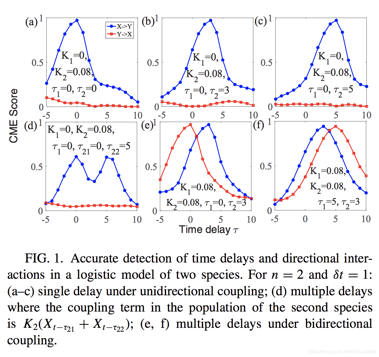
It is straightforward to show $0\le s\le 1$. The larger the value of $s$, the stronger the driving force from $x(t-\tau )$ to $y(t)$. In a plot of $s(\tau )$, if there is a peak at ${\tau }_k\in \Gamma$, the time delay from $X$ to $Y$ can be identified as ${\tau }_k$.
可以理解为如果$x$是以延迟${\tau }_k$作用于$y$，那么当$y$的情况（$Y$）类似时，${\tau }_k$之前的$x$（也就是$z$）的情况($Z$)也应该类似（协方差大，相关性强），形式上和pearson相关系数一样。

RESULTS

To validate our CME method, we begin with a discrete-time logistic model of two non-identical species:

$$X_{t+1}=X_t({\gamma }_x-{\gamma }_x{X}_t-K_1{Y}_{t-{\tau }_1})$$

$$Y_{t+1}=Y_t({\gamma }_y-{\gamma }_y{Y}_t-K_2{X}_{t-{\tau }_2})$$

where ${\gamma }_x=3.78,{\gamma }_y=3.77$, $K_1$ and $K_2$ are the coupling parameters, and ${\tau }_1$ and ${\tau }_2$ are the intrinsic time delays that we aim to determine from time series.

后面也举了几个微分方程的例子。

疑问：他所举例都是两个节点的连接，并没有把方法运用到网络中。

第二篇工作

Randomly distributed embedding making short-term high-dimensional data predictable

Abstract

In this work, we propose a model-free framework, named randomly distributed embedding (RDE), to achieve accurate future state prediction based on short-term high-dimensional data.
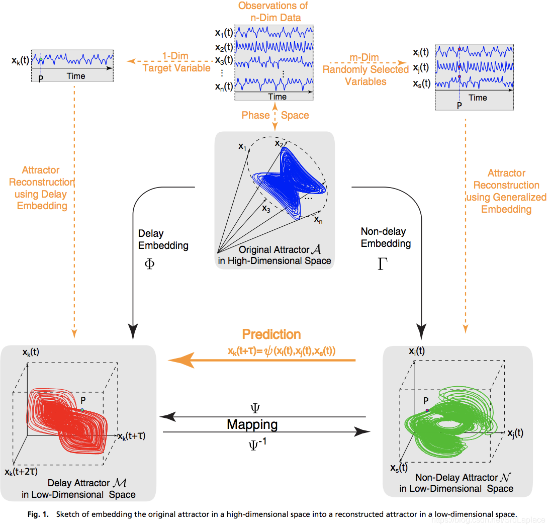
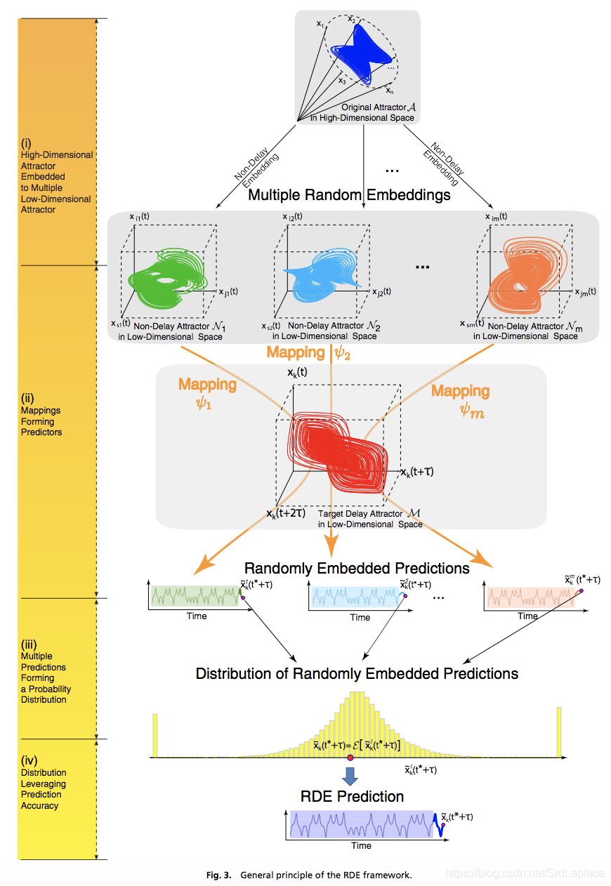
From the observed data of high-dimensional variables, the RDE framework randomly generates a sufficient number of low-dimensional “nondelay embeddings” and maps each of them to a “delay embedding,” which is constructed from the data of a to be predicted target variable.
Any of these mappings can perform as a low-dimensional weak predictor for future state prediction, and all of such mappings generate a distribution of predicted future states.

用机器学习embedding的思想，把随机选取若干个变量当作特征，预测指定节点的值，然后进行embedding。

RDE Framework

For each index tuple $l=(l_i,l_2,...,l_L)$, a component of such a mapping, denoted by ${\varphi }_l$ , can be obtained as a predictor for the target variable $x_k(t)$ in the form of

$$x_k(t+\tau )={\varphi }_l(x_{l_1}(t),x_{l_2}(t),...,x_{l_L}(t))$$

Notice that $L$ is much lower than the dimension $n$ of the entire system. Then, typical approximation frameworks with usual fitting algorithms could be used to implement this predictor. In this paper, we apply the Gaussian Process Regression method to fit each ${\varphi }_l$ .

Specifically, better prediction can be estimated by

$${\hat{x}}_k(t+\tau )=E[{\hat{x}}_k^l(t+\tau )]$$

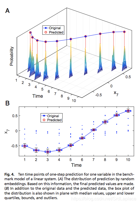
where $E[\cdot ]$ represents an estimation based on the available probability information of the random variable${\hat{x}}_k^l$. A straightforward scheme to obtain this estimation is to use the expectation of the distribution as the final prediction value [i.e., ${\hat{x}}_k(t+\tau )=\int xp(x)dx$ , where $p(x)$ denotes the probability density function of the random variable ${\hat{x}}_k^l$].

In light of the feature bagging strategy in machine learning, each random embedding is treated as a feature, and thus, the final prediction value is estimated by the aggregated average of the selected features: that is,

$$x_k(t+\tau )=\sum _i{w}_i{\hat{x}}_k^l(t+\tau )$$

where each $w_i$ is a weight related to the in-sample fitting error of ${\varphi }_i$ and the equation represents the best fitting errors for the final prediction.

Methods

Given time series data sampled from $n$ variables of a system with length $m$ (i.e., $x(t)\in R_n,t=t_1,t_2,...,t_m$, where $ti=t_{I-1}+\tau$), one can estimate the box-counting dimension $d$ of the system’s dynamics and choose embedding dimension $L>2d$. Assume that the target variable to be predicted is represented as $x_k$. The RDE algorithm is listed as follows:

• Randomly pick s tuples from $(1,2,\dots ,n)$ with replacement, and each tuple contains $L$ numbers.
• For the $l$th tuple $(l_1,l_2,\dots ,l_L)$, fit a predictor ${\varphi }_i$ so as to minimize ${\sum }_{I=1}^{m-1}||x_k(t_i+\tau )-{\varphi }_l(x_{l_1}(t_i),x_{l_2}(t_i),\dots ,x_{l_L}(ti)||$. Standard fitting algorithms could be adopted. In this paper, Gaussian Process Regression is used.
• Use each predictor ${\varphi }_l$ , and make one-step prediction ${\hat{x}}_k^l(t^{\ast }+\tau )={\varphi }_l(x_{l_1}(t^{\ast }),x_{l_2}(t^{\ast }),\dots ,x_{l_L}(t^{\ast })$ for a specific future time $t^{\ast }+\tau$.
• Multiple predicted values form a set {x^kl(t∗+τ)}\{\hat{x}^l_k(t^* + \tau)\}{x^kl​(t∗+τ)}. Exclude the outliers from the set, and use the Kernel Density Estimation method to approximate the probability density function $p(x)$ of its distribution.
• 将预测值的分布的平均当作是预测值. Otherwise, calculate the in-sample prediction error ${\delta }_l$ for the fitted ${\varphi }_l$ using the leave-one-out method. Based on the rank of the in-sample error, $r$ best tuples are picked out, and the final prediction is given by the aggregated average in the form of $x_k(t+\tau )={\sum }_i^r{w}_i{\hat{x}}_k^l(t+\tau )$, where the weight $w_i=\frac{exp(-{\delta }_i/{\delta }_1)}{{\sum }_{j}exp(-{\delta }_j/{\delta }_1)}$ .

Result

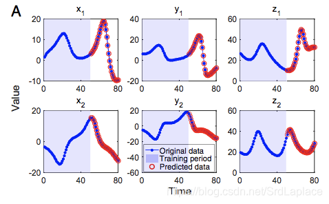
As particularly shown in Fig. 1, with the n-dimensional time series data $x_i(t),i=1,2,...,n$, two kinds of 3D (threedimensional) attractors can be reconstructed.

加噪声和选取不同的训练时间长度对结果的影响

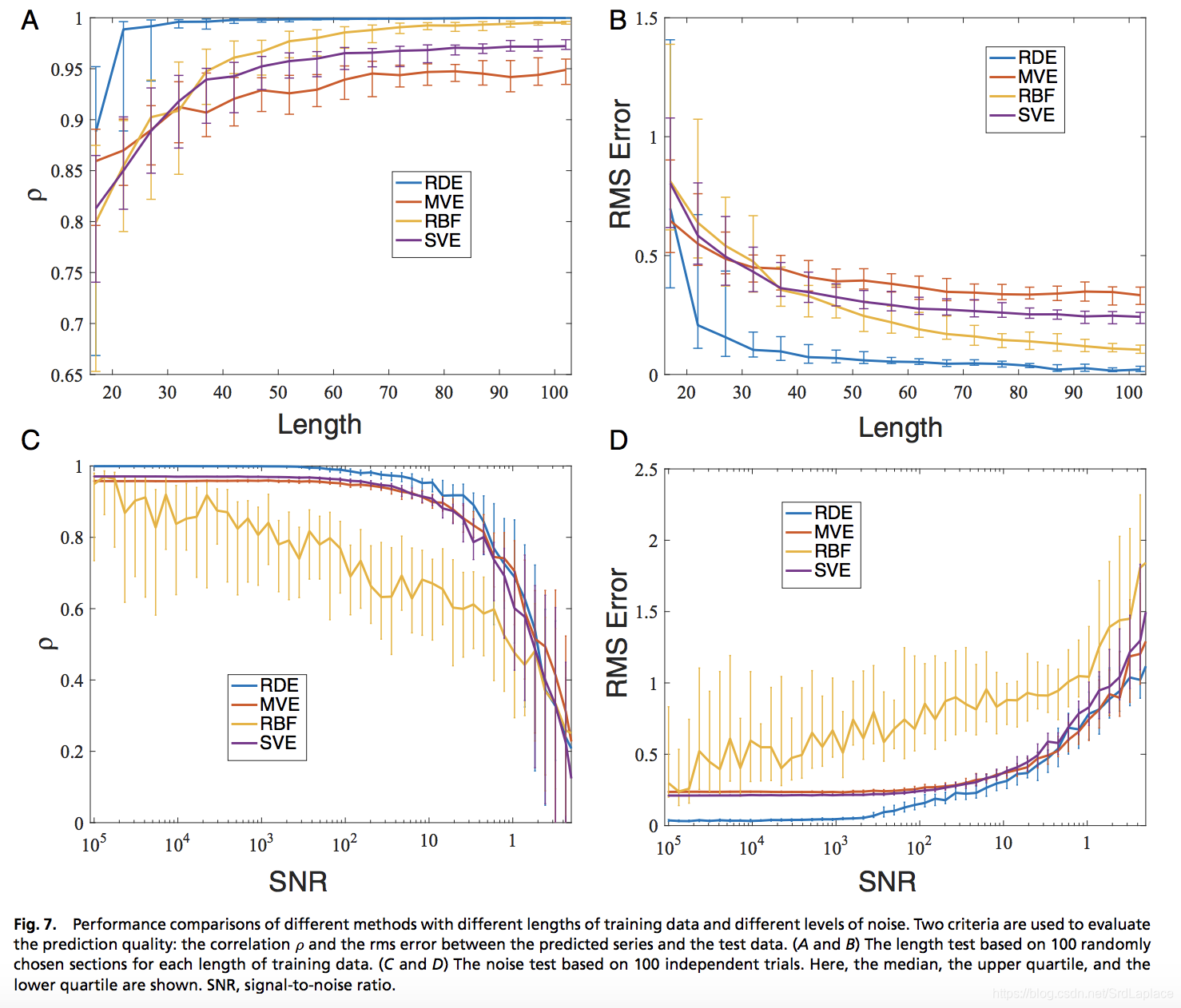
SNR 是信噪比；RDE 是本文的方法（randomly distributed embedding）；MVE 是 multiview embedding method；RBF表示RDE采用RBF (radial basis function) network来进行预测的方法； SVE 是 the classic single-variable embedding method。

疑问：混沌系统具有长时间不可预测性，如果不准确预测参数，长时间的预测是不可能的。文章选取的预测时间都很短，也没有探究随着时间的推移误差变化情况；所加噪声不大的情况下，效果也变差的比较快。