【2021.05--集成学习（下）-Task15】蒸汽预测案例

本次 DataWhale 第二十五期组队学习，其开源内容的链接为：https://github.com/datawhalechina/team-learning-data-mining/tree/master/EnsembleLearning

导入包

import warnings
warnings.filterwarnings("ignore")
import matplotlib.pyplot as plt
import seaborn as sns

# 模型
import pandas as pd
import numpy as np
from scipy import stats
from sklearn.model_selection import train_test_split
from sklearn.model_selection import GridSearchCV, RepeatedKFold, cross_val_score,cross_val_predict,KFold
from sklearn.metrics import make_scorer,mean_squared_error
from sklearn.linear_model import LinearRegression, Lasso, Ridge, ElasticNet
from sklearn.svm import LinearSVR, SVR
from sklearn.neighbors import KNeighborsRegressor
from sklearn.ensemble import RandomForestRegressor, GradientBoostingRegressor,AdaBoostRegressor
from xgboost import XGBRegressor
from sklearn.preprocessing import PolynomialFeatures,MinMaxScaler,StandardScaler

读取数据

data_train = pd.read_csv('train.txt',sep = '\t')
data_test = pd.read_csv('test.txt',sep = '\t')
data_train.shape, data_test.shape

((2888, 39), (1925, 38))

#合并训练数据和测试数据
data_train["oringin"]="train"
data_test["oringin"]="test"
data_all=pd.concat([data_train,data_test],axis=0,ignore_index=True)
#显示前5条数据
data_all.head()

	V0	V1	V2	V3	V4	V5	V6	V7	V8	V9	...	V30	V31	V32	V33	V34	V35	V36	V37	target	oringin
0	0.566	0.016	-0.143	0.407	0.452	-0.901	-1.812	-2.360	-0.436	-2.114	...	0.109	-0.615	0.327	-4.627	-4.789	-5.101	-2.608	-3.508	0.175	train
1	0.968	0.437	0.066	0.566	0.194	-0.893	-1.566	-2.360	0.332	-2.114	...	0.124	0.032	0.600	-0.843	0.160	0.364	-0.335	-0.730	0.676	train
2	1.013	0.568	0.235	0.370	0.112	-0.797	-1.367	-2.360	0.396	-2.114	...	0.361	0.277	-0.116	-0.843	0.160	0.364	0.765	-0.589	0.633	train
3	0.733	0.368	0.283	0.165	0.599	-0.679	-1.200	-2.086	0.403	-2.114	...	0.417	0.279	0.603	-0.843	-0.065	0.364	0.333	-0.112	0.206	train
4	0.684	0.638	0.260	0.209	0.337	-0.454	-1.073	-2.086	0.314	-2.114	...	1.078	0.328	0.418	-0.843	-0.215	0.364	-0.280	-0.028	0.384	train

5 rows × 40 columns

探索数据分布

这里因为是传感器的数据，即连续变量，所以使用 kdeplot(核密度估计图) 进行数据的初步分析，即EDA。

for column in data_all.columns[0:-2]:
    #核密度估计(kernel density estimation)是在概率论中用来估计未知的密度函数，属于非参数检验方法之一。通过核密度估计图可以比较直观的看出数据样本本身的分布特征。
    g = sns.kdeplot(data_all[column][(data_all["oringin"] == "train")], color="Red", shade = True)
    g = sns.kdeplot(data_all[column][(data_all["oringin"] == "test")], ax =g, color="Blue", shade= True)
    g.set_xlabel(column)
    g.set_ylabel("Frequency")
    g = g.legend(["train","test"])
    plt.show()

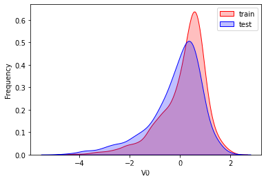
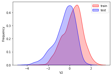
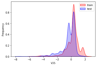
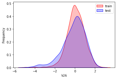
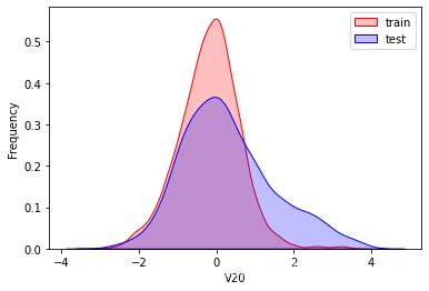
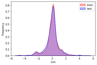
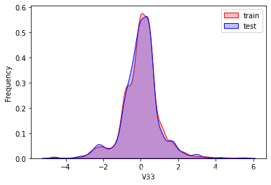
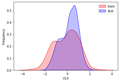
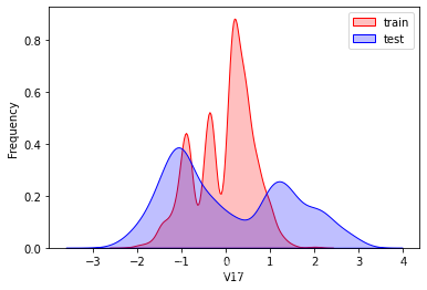
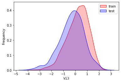
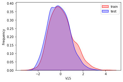
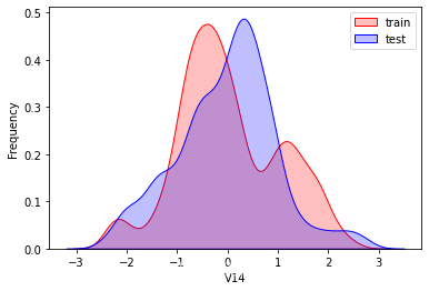
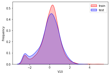
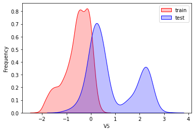
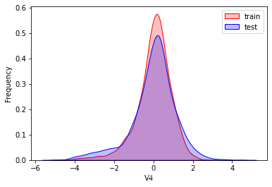
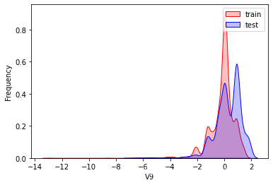
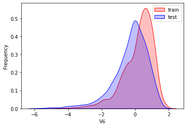
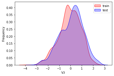
可以看出V2、V5、V9、V14、V17、V20、V21、V22等8个特征在分布上有较大差异。

查看特征之间的相关性（相关程度）

data_train1=data_all[data_all["oringin"]=="train"].drop("oringin",axis=1)
plt.figure(figsize=(20, 16))  # 指定绘图对象宽度和高度
colnm = data_train1.columns.tolist()  # 列表头
mcorr = data_train1[colnm].corr(method="spearman")  # 相关系数矩阵，即给出了任意两个变量之间的相关系数
mask = np.zeros_like(mcorr, dtype=np.bool)  # 构造与mcorr同维数矩阵 为bool型
mask[np.triu_indices_from(mask)] = True  # 角分线右侧为True
cmap = sns.diverging_palette(220, 10, as_cmap=True)  # 返回matplotlib colormap对象，调色板
g = sns.heatmap(mcorr, mask=mask, cmap=cmap, square=True, annot=True, fmt='0.2f')  # 热力图（看两两相似度）
plt.show()

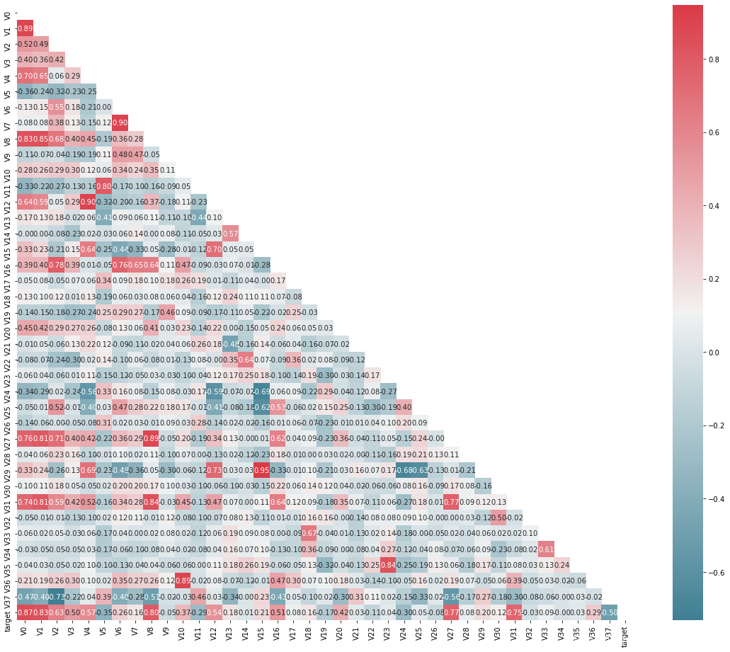
进行降维操作，即将相关性的绝对值小于阈值的特征进行删除

threshold = 0.1
corr_matrix = data_train1.corr().abs()
drop_col=corr_matrix[corr_matrix["target"]<threshold].index # 与target相关性小于阈值的列删除
data_all.drop(drop_col,axis=1,inplace=True)
data_all.shape

(4813, 33)

进行归一化操作

cols_numeric=list(data_all.columns)
cols_numeric.remove("oringin")
# 自定义函数进行0-1缩放
def scale_minmax(col):
    return (col-col.min())/(col.max()-col.min())
scale_cols = [col for col in cols_numeric if col!='target']
data_all[scale_cols] = data_all[scale_cols].apply(scale_minmax,axis=0)
data_all[scale_cols].describe()

	V0	V1	V2	V3	V4	V5	V6	V7	V8	V9	...	V23	V24	V27	V28	V29	V30	V31	V35	V36	V37
count	4813.000000	4813.000000	4813.000000	4813.000000	4813.000000	4813.000000	4813.000000	4813.000000	4813.000000	4813.000000	...	4813.000000	4813.000000	4813.000000	4813.000000	4813.000000	4813.000000	4813.000000	4813.000000	4813.000000	4813.000000
mean	0.694172	0.721357	0.602300	0.603139	0.523743	0.407246	0.748823	0.745740	0.715607	0.879536	...	0.744438	0.356712	0.881401	0.342653	0.388683	0.589459	0.792709	0.762873	0.332385	0.545795
std	0.144198	0.131443	0.140628	0.152462	0.106430	0.186636	0.132560	0.132577	0.118105	0.068244	...	0.134085	0.265512	0.128221	0.140731	0.133475	0.130786	0.102976	0.102037	0.127456	0.150356
min	0.000000	0.000000	0.000000	0.000000	0.000000	0.000000	0.000000	0.000000	0.000000	0.000000	...	0.000000	0.000000	0.000000	0.000000	0.000000	0.000000	0.000000	0.000000	0.000000	0.000000
25%	0.626676	0.679416	0.514414	0.503888	0.478182	0.298432	0.683324	0.696938	0.664934	0.852903	...	0.719362	0.040616	0.888575	0.278778	0.292445	0.550092	0.761816	0.727273	0.270584	0.445647
50%	0.729488	0.752497	0.617072	0.614270	0.535866	0.382419	0.774125	0.771974	0.742884	0.882377	...	0.788817	0.381736	0.916015	0.279904	0.375734	0.594428	0.815055	0.800020	0.347056	0.539317
75%	0.790195	0.799553	0.700464	0.710474	0.585036	0.460246	0.842259	0.836405	0.790835	0.941189	...	0.792706	0.574728	0.932555	0.413031	0.471837	0.650798	0.852229	0.800020	0.414861	0.643061
max	1.000000	1.000000	1.000000	1.000000	1.000000	1.000000	1.000000	1.000000	1.000000	1.000000	...	1.000000	1.000000	1.000000	1.000000	1.000000	1.000000	1.000000	1.000000	1.000000	1.000000

8 rows × 31 columns

特征工程

绘图显示Box-Cox变换对数据分布影响，Box-Cox用于连续的响应变量不满足正态分布的情况。在进行Box-Cox变换之后，可以一定程度上减小不可观测的误差和预测变量的相关性。

fcols = 6
frows = len(cols_numeric)-1
plt.figure(figsize=(4*fcols,4*frows))
i=0

for var in cols_numeric:
    if var!='target':
        dat = data_all[[var, 'target']].dropna()  # 与target的相关系数
        
        i+=1
        plt.subplot(frows,fcols,i)
        sns.distplot(dat[var] , fit=stats.norm);
        plt.title(var+' Original')
        plt.xlabel('')
        
        i+=1
        plt.subplot(frows,fcols,i)
        _=stats.probplot(dat[var], plot=plt)
        plt.title('skew='+'{:.4f}'.format(stats.skew(dat[var])))
        plt.xlabel('')
        plt.ylabel('')
        
        i+=1
        plt.subplot(frows,fcols,i)
        plt.plot(dat[var], dat['target'],'.',alpha=0.5)
        plt.title('corr='+'{:.2f}'.format(np.corrcoef(dat[var], dat['target'])[0][1]))
 
        i+=1
        plt.subplot(frows,fcols,i)
        trans_var, lambda_var = stats.boxcox(dat[var].dropna()+1)
        trans_var = scale_minmax(trans_var)      
        sns.distplot(trans_var , fit=stats.norm);
        plt.title(var+' Tramsformed')
        plt.xlabel('')
        
        i+=1
        plt.subplot(frows,fcols,i)
        _=stats.probplot(trans_var, plot=plt)
        plt.title('skew='+'{:.4f}'.format(stats.skew(trans_var)))
        plt.xlabel('')
        plt.ylabel('')
        
        i+=1
        plt.subplot(frows,fcols,i)
        plt.plot(trans_var, dat['target'],'.',alpha=0.5)
        plt.title('corr='+'{:.2f}'.format(np.corrcoef(trans_var,dat['target'])[0][1]))

# 进行Box-Cox变换
cols_transform=data_all.columns[0:-2]
for col in cols_transform:   
    # transform column
    data_all.loc[:,col], _ = stats.boxcox(data_all.loc[:,col]+1)
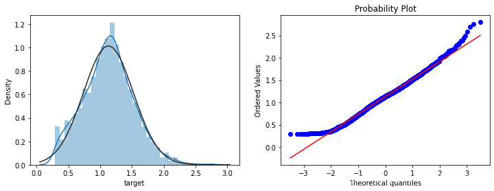
print(data_all.target.describe())
plt.figure(figsize=(12,4))
plt.subplot(1,2,1)
sns.distplot(data_all.target.dropna() , fit=stats.norm);
plt.subplot(1,2,2)
_=stats.probplot(data_all.target.dropna(), plot=plt)

count    2888.000000
mean        0.126353
std         0.983966
min        -3.044000
25%        -0.350250
50%         0.313000
75%         0.793250
max         2.538000
Name: target, dtype: float64

使用对数变换target目标值提升特征数据的正太性

sp = data_train.target
data_train.target1 =np.power(1.5,sp)
print(data_train.target1.describe())

plt.figure(figsize=(12,4))
plt.subplot(1,2,1)
sns.distplot(data_train.target1.dropna(),fit=stats.norm);
plt.subplot(1,2,2)
_=stats.probplot(data_train.target1.dropna(), plot=plt)

count    2888.000000
mean        1.129957
std         0.394110
min         0.291057
25%         0.867609
50%         1.135315
75%         1.379382
max         2.798463
Name: target, dtype: float64

模型构建以及集成学习

构建训练集和测试集

# function to get training samples
def get_training_data():
    # extract training samples
    from sklearn.model_selection import train_test_split
    df_train = data_all[data_all["oringin"]=="train"]
    df_train["label"]=data_train.target1
    # split SalePrice and features
    y = df_train.target
    X = df_train.drop(["oringin","target","label"],axis=1)
    X_train,X_valid,y_train,y_valid=train_test_split(X,y,test_size=0.3,random_state=100)
    return X_train,X_valid,y_train,y_valid

# extract test data (without SalePrice)
def get_test_data():
    df_test = data_all[data_all["oringin"]=="test"].reset_index(drop=True)
    return df_test.drop(["oringin","target"],axis=1)

rmse、mse的评价函数

from sklearn.metrics import make_scorer
# metric for evaluation
def rmse(y_true, y_pred):
    diff = y_pred - y_true
    sum_sq = sum(diff**2)    
    n = len(y_pred)   
    return np.sqrt(sum_sq/n)

def mse(y_ture,y_pred):
    return mean_squared_error(y_ture,y_pred)

# scorer to be used in sklearn model fitting
rmse_scorer = make_scorer(rmse, greater_is_better=False) 

#输入的score_func为记分函数时，该值为True（默认值）；输入函数为损失函数时，该值为False
mse_scorer = make_scorer(mse, greater_is_better=False)

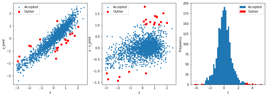
寻找离群值，并删除

# function to detect outliers based on the predictions of a model
def find_outliers(model, X, y, sigma=3):

    # predict y values using model
    model.fit(X,y)
    y_pred = pd.Series(model.predict(X), index=y.index)
        
    # calculate residuals between the model prediction and true y values
    resid = y - y_pred
    mean_resid = resid.mean()
    std_resid = resid.std()

    # calculate z statistic, define outliers to be where |z|>sigma
    z = (resid - mean_resid)/std_resid    
    outliers = z[abs(z)>sigma].index
    
    # print and plot the results
    print('R2=',model.score(X,y))
    print('rmse=',rmse(y, y_pred))
    print("mse=",mean_squared_error(y,y_pred))
    print('---------------------------------------')

    print('mean of residuals:',mean_resid)
    print('std of residuals:',std_resid)
    print('---------------------------------------')

    print(len(outliers),'outliers:')
    print(outliers.tolist())

    plt.figure(figsize=(15,5))
    ax_131 = plt.subplot(1,3,1)
    plt.plot(y,y_pred,'.')
    plt.plot(y.loc[outliers],y_pred.loc[outliers],'ro')
    plt.legend(['Accepted','Outlier'])
    plt.xlabel('y')
    plt.ylabel('y_pred');

    ax_132=plt.subplot(1,3,2)
    plt.plot(y,y-y_pred,'.')
    plt.plot(y.loc[outliers],y.loc[outliers]-y_pred.loc[outliers],'ro')
    plt.legend(['Accepted','Outlier'])
    plt.xlabel('y')
    plt.ylabel('y - y_pred');

    ax_133=plt.subplot(1,3,3)
    z.plot.hist(bins=50,ax=ax_133)
    z.loc[outliers].plot.hist(color='r',bins=50,ax=ax_133)
    plt.legend(['Accepted','Outlier'])
    plt.xlabel('z')
    
    return outliers

# get training data
X_train, X_valid,y_train,y_valid = get_training_data()
test=get_test_data()

# find and remove outliers using a Ridge model
outliers = find_outliers(Ridge(), X_train, y_train)
X_outliers=X_train.loc[outliers]
y_outliers=y_train.loc[outliers]
X_t=X_train.drop(outliers)
y_t=y_train.drop(outliers)

R2= 0.8819987457476228
rmse= 0.34138451265265296
mse= 0.11654338547908945
---------------------------------------
mean of residuals: 1.2195423625273862e-16
std of residuals: 0.341469003314175
---------------------------------------
21 outliers:
[2863, 1145, 2697, 2528, 1882, 2645, 691, 1874, 2647, 884, 2696, 2668, 1310, 1901, 1979, 1458, 2769, 2002, 2669, 1040, 1972]

进行模型的训练

def get_trainning_data_omitoutliers():
    #获取训练数据省略异常值
    y=y_t.copy()
    X=X_t.copy()
    return X,y

def train_model(model, param_grid=[], X=[], y=[], 
                splits=5, repeats=5):

    # 获取数据
    if len(y)==0:
        X,y = get_trainning_data_omitoutliers()
        
    # 交叉验证
    rkfold = RepeatedKFold(n_splits=splits, n_repeats=repeats)
    
    # 网格搜索最佳参数
    if len(param_grid)>0:
        gsearch = GridSearchCV(model, param_grid, cv=rkfold,
                               scoring="neg_mean_squared_error",
                               verbose=1, return_train_score=True)

        # 训练
        gsearch.fit(X,y)

        # 最好的模型
        model = gsearch.best_estimator_        
        best_idx = gsearch.best_index_

        # 获取交叉验证评价指标
        grid_results = pd.DataFrame(gsearch.cv_results_)
        cv_mean = abs(grid_results.loc[best_idx,'mean_test_score'])
        cv_std = grid_results.loc[best_idx,'std_test_score']

    # 没有网格搜索  
    else:
        grid_results = []
        cv_results = cross_val_score(model, X, y, scoring="neg_mean_squared_error", cv=rkfold)
        cv_mean = abs(np.mean(cv_results))
        cv_std = np.std(cv_results)
    
    # 合并数据
    cv_score = pd.Series({'mean':cv_mean,'std':cv_std})

    # 预测
    y_pred = model.predict(X)
    
    # 模型性能的统计数据        
    print('----------------------')
    print(model)
    print('----------------------')
    print('score=',model.score(X,y))
    print('rmse=',rmse(y, y_pred))
    print('mse=',mse(y, y_pred))
    print('cross_val: mean=',cv_mean,', std=',cv_std)
    
    # 残差分析与可视化
    y_pred = pd.Series(y_pred,index=y.index)
    resid = y - y_pred
    mean_resid = resid.mean()
    std_resid = resid.std()
    z = (resid - mean_resid)/std_resid    
    n_outliers = sum(abs(z)>3)
    outliers = z[abs(z)>3].index
    
    return model, cv_score, grid_results

# 定义训练变量存储数据
opt_models = dict()
score_models = pd.DataFrame(columns=['mean','std'])
splits=5
repeats=5

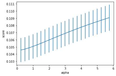
model = 'Ridge'  #可替换，见案例分析一的各种模型
opt_models[model] = Ridge() #可替换，见案例分析一的各种模型
alph_range = np.arange(0.25,6,0.25)
param_grid = {'alpha': alph_range}

opt_models[model],cv_score,grid_results = train_model(opt_models[model], param_grid=param_grid, 
                                              splits=splits, repeats=repeats)

cv_score.name = model
score_models = score_models.append(cv_score)

plt.figure()
plt.errorbar(alph_range, abs(grid_results['mean_test_score']),
             abs(grid_results['std_test_score'])/np.sqrt(splits*repeats))
plt.xlabel('alpha')
plt.ylabel('score')

Fitting 25 folds for each of 23 candidates, totalling 575 fits
----------------------
Ridge(alpha=0.25)
----------------------
score= 0.8970035888674313
rmse= 0.3171387115307921
mse= 0.1005769623514108
cross_val: mean= 0.10456455890924238 , std= 0.008398143726644422





Text(0, 0.5, 'score')

# 测试不同模型 -- 先查看参数啊
LinearRegression().get_params().keys()

dict_keys(['copy_X', 'fit_intercept', 'n_jobs', 'normalize', 'positive'])

model = 'LinearRegression'  #可替换，见案例分析一的各种模型
opt_models[model] = LinearRegression() #可替换，见案例分析一的各种模型
normalize_range = np.arange(0,2,1)
param_grid = {'normalize': normalize_range}

opt_models[model],cv_score,grid_results = train_model(opt_models[model], param_grid=param_grid, 
                                              splits=splits, repeats=repeats)

cv_score.name = model
score_models = score_models.append(cv_score)

plt.figure()
plt.errorbar(normalize_range, abs(grid_results['mean_test_score']),
             abs(grid_results['std_test_score'])/np.sqrt(splits*repeats))
plt.xlabel('normalize')
plt.ylabel('score')

Fitting 25 folds for each of 2 candidates, totalling 50 fits
----------------------
LinearRegression(normalize=0)
----------------------
score= 0.8971017130584396
rmse= 0.31698760726209607
mse= 0.10048114315774888
cross_val: mean= 0.10472998637691651 , std= 0.005702243997201932





Text(0, 0.5, 'score')

# 预测函数
def model_predict(test_data,test_y=[]):
    i=0
    y_predict_total=np.zeros((test_data.shape[0],))
    for model in opt_models.keys():
        if model!="LinearSVR" and model!="KNeighbors":
            y_predict=opt_models[model].predict(test_data)
            y_predict_total+=y_predict
            i+=1
        if len(test_y)>0:
            print("{}_mse:".format(model),mean_squared_error(y_predict,test_y))
    y_predict_mean=np.round(y_predict_total/i,6)
    if len(test_y)>0:
        print("mean_mse:",mean_squared_error(y_predict_mean,test_y))
    else:
        y_predict_mean=pd.Series(y_predict_mean)
        return y_predict_mean

进行模型的预测以及结果的保存

y_ = model_predict(test)
y_.to_csv('predict.txt',header = None,index = False)