Course 2 改善深层神经网络 Week 1 一维函数和多层神经网络的梯度检查

一维与多层神经网梯度检查

最新推荐文章于 2023-12-27 18:56:28 发布

原创最新推荐文章于 2023-12-27 18:56:28 发布 · 316 阅读

0 ·

CC 4.0 BY-SA版权

文章标签：

#python #深度学习 #梯度检查 #GradientChecking

深度学习专栏收录该内容

6 篇文章

订阅专栏

本文介绍了一维函数与多层神经网络的梯度检查方法，包括梯度定义、一维函数梯度检查流程及多层神经网络参数梯度检查的具体实现。

一维函数的梯度检查

软件包导入

import numpy as np
import matplotlib.pyplot as plt

反向传播计算梯度 $∂J∂θ\frac{\partial J}{\partial \theta}$ , $θ\theta$ 表示模型中的参数，使用前向传播和损失函数计算 $J$ ，因为向前传播相对容易实现，所以您确信自己得到了正确的结果，所以您几乎100％确定您正确计算了 $J$ 。因此，您可以使用您的代码来计算 $J$ 验证反向传播计算的梯度 $∂J∂θ\frac{\partial J}{\partial \theta}$ 。
导数（或梯度）的定义：
$\frac{\partial J}{\partial \theta} = \lim_{\varepsilon \to 0} \frac{J(\theta + \varepsilon) - J(\theta - \varepsilon)}{2 \varepsilon}$

一维函数传播示意图
在这里插入图片描述
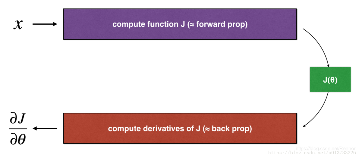
首先需用 $x$ 前向传播计算得到 $\theta * x$ ，然后由反向传播计算得到 $∂J∂θ\frac{\partial J}{\partial \theta}$

def forward_propagation(x, theta):
    '''
    实现一元函数的线性前向传播（计算J） J(theta)= theta * X
    :param x: 输入
    :param theta: θ，乘数
    :return:
        J：函数J(θ)= θ * X的值
    '''
    J = np.dot(theta, x)
    return J
def backward_propagation(x, theta):
    '''
    计算J(theta)= theta * X相对于θ的导数
    :param x: 输入
    :param theta: θ，实数
    :return:
        dtheta:相对于θc的成本梯度
    '''
    dtheta = x

    return dtheta

一维函数梯度检查

梯度检查的步骤如下，首先计算线性误差"gradapprox"，精度是 $ε\varepsilon$ .
1. $θ+=θ+ε\theta^{+} = \theta + \varepsilon$
2. $θ−=θ−ε\theta^{-} = \theta - \varepsilon$
3. $J+=J(θ+)J^{+} = J(\theta^{+})$
4. $J−=J(θ−)J^{-} = J(\theta^{-})$
5. $\frac{J^{+} - J^{-}}{2 \varepsilon}$

反向传播计算得到各个值的梯度值 “grad”，然后与"gradapprox"计算出两者的欧几里得范数：
$\frac {\mid\mid grad - gradapprox \mid\mid_2}{\mid\mid grad \mid\mid_2 + \mid\mid gradapprox \mid\mid_2} \tag{2}$
需要计算上面的公式:
- 1’. 计算分子用 np.linalg.norm(...)
- 2’. 计算分母用两次np.linalg.norm(...)
- 3’. 然后相除
  当difference小于 $10^{-7}$ 时，通常认为计算结果是正确的。

def gradient_check(x, theta, epsilon=1e-7):
    """
    实现微分和导数间的计算，进行梯度检验
    Arguments:
        x：实值输入
        theta ：参数，也是实值
        epsilon ：微小偏移以计算近似梯度

    Returns:
        difference：近似梯度gradapprox和后向传播梯度grad之间的差值
    """

    # 计算gradapprox
    thetaplus = theta + epsilon  # Step 1
    thetaminus = theta - epsilon  # Step 2
    J_plus = forward_propagation(x, thetaplus)  # Step 3
    J_minus = forward_propagation(x, thetaminus)  # Step 4
    gradapprox = (J_plus - J_minus) / (2 * epsilon)  # Step 5

    # 检查gradapprox是否和反向传播backward_propagation()输出grad相接近
    grad = backward_propagation(x, theta)

    numerator = np.linalg.norm(grad - gradapprox)  # Step 1'
    denominator = np.linalg.norm(grad) + np.linalg.norm(gradapprox)  # Step 2'
    difference = numerator / denominator  # Step 3'

    if difference < 1e-7:
        print("梯度检查：梯度正常")
    else:
        print("梯度检查：超出阈值")

    return difference

测试一下

#测试gradient_check
print("-----------------测试gradient_check-----------------")
x, theta = 2, 4
difference = gradient_check(x, theta)
print("difference = " + str(difference))

测试结果

-----------------测试gradient_check-----------------
梯度检查：梯度正常!
difference = 2.91933588329e-10

多层神经网络参数的梯度检查

在这里插入图片描述

前向传播计算

def sigmoid(x):
    """
    Compute the sigmoid of x

    Arguments:
    x -- A scalar or numpy array of any size.

    Return:
    s -- sigmoid(x)
    """
    s = 1 / (1 + np.exp(-x))
    return s


def relu(x):
    """
    Compute the relu of x

    Arguments:
    x -- A scalar or numpy array of any size.

    Return:
    s -- relu(x)
    """
    s = np.maximum(0, x)

    return s

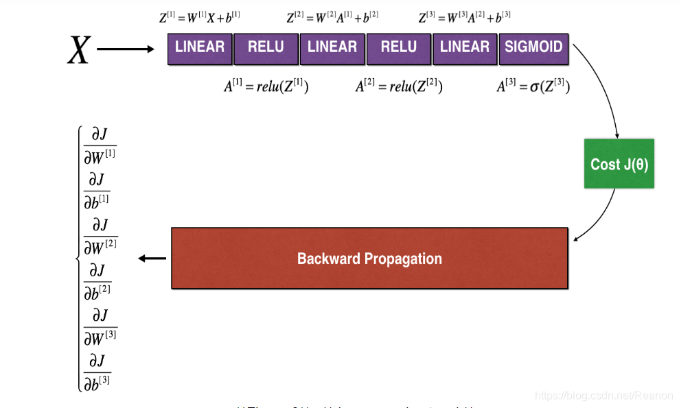
def forward_propagation_n(X, Y, parameters):
    """
    实现图中的前向传播（并计算成本）。
    参数：
        X - 训练集为m个例子
        Y -  m个示例的标签
        parameters - 包含参数“W1”，“b1”，“W2”，“b2”，“W3”，“b3”的python字典：
            W1  - 权重矩阵，维度为（5,4）
            b1  - 偏向量，维度为（5,1）
            W2  - 权重矩阵，维度为（3,5）
            b2  - 偏向量，维度为（3,1）
            W3  - 权重矩阵，维度为（1,3）
            b3  - 偏向量，维度为（1,1）
    返回：
        cost - 成本函数（logistic）
    """
    m = X.shape[1]
    W1 = parameters["W1"]
    b1 = parameters["b1"]
    W2 = parameters["W2"]
    b2 = parameters["b2"]
    W3 = parameters["W3"]
    b3 = parameters["b3"]

    # LINEAR -> RELU -> LINEAR -> RELU -> LINEAR -> SIGMOID
    Z1 = np.dot(W1, X) + b1
    A1 = relu(Z1)
    Z2 = np.dot(W2, A1) + b2
    A2 = relu(Z2)
    Z3 = np.dot(W3, A2) + b3
    A3 = sigmoid(Z3)
    # 计算成本
    logprobs = np.multiply(-np.log(A3), Y) + np.multiply(-np.log(1 - A3), 1 - Y)
    cost = (1 / m) * np.sum(logprobs)
    cache = (Z1, A1, W1, b1, Z2, A2, W2, b2, Z3, A3, W3, b3)
    return cost, cache

反向传播

因为这里层数比较浅，没有直接用到relu_backward()和sigmoid_backward()。

def backward_propagation_n(X, Y, cache):
    """
    实现图中所示的反向传播。
    参数：
        X - 输入数据点（输入节点数量，1）
        Y - 标签
        cache - 来自forward_propagation_n（）的cache输出
    返回：
        gradients - 一个字典，其中包含与每个参数、激活和激活前变量相关的成本梯度。
    """
    m = X.shape[1]
    (Z1, A1, W1, b1, Z2, A2, W2, b2, Z3, A3, W3, b3) = cache

    dZ3 = A3 - Y # 需要考究一下
    dW3 = (1. / m) * np.dot(dZ3, A2.T)
    dW3 = 1. / m * np.dot(dZ3, A2.T)
    db3 = 1. / m * np.sum(dZ3, axis=1, keepdims=True)

    dA2 = np.dot(W3.T, dZ3)
    dZ2 = np.multiply(dA2, np.int64(A2 > 0))
    # dW2 = 1. / m * np.dot(dZ2, A1.T) * 2  # Should not multiply by 2
    dW2 = 1. / m * np.dot(dZ2, A1.T)
    db2 = 1. / m * np.sum(dZ2, axis=1, keepdims=True)

    dA1 = np.dot(W2.T, dZ2)
    dZ1 = np.multiply(dA1, np.int64(A1 > 0))
    dW1 = 1. / m * np.dot(dZ1, X.T)
    # db1 = 4. / m * np.sum(dZ1, axis=1, keepdims=True) # Should not multiply by 4
    db1 = 1. / m * np.sum(dZ1, axis=1, keepdims=True)
    gradients = {"dZ3": dZ3, "dW3": dW3, "db3": db3,
                 "dA2": dA2, "dZ2": dZ2, "dW2": dW2, "db2": db2,
                 "dA1": dA1, "dZ1": dZ1, "dW1": dW1, "db1": db1}
    return gradients

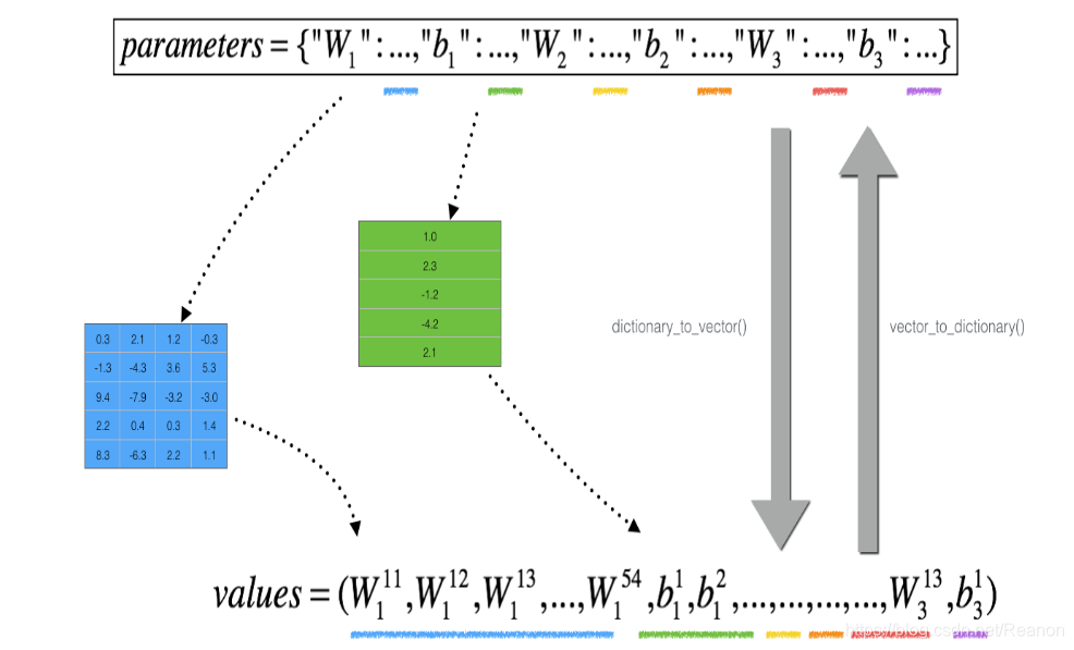
参数格式转换

如果想比较"gradapprox" 与反向传播计算的梯度。该公式仍然是：
$\frac{\partial J}{\partial \theta} = \lim_{\varepsilon \to 0} \frac{J(\theta + \varepsilon) - J(\theta - \varepsilon)}{2 \varepsilon}$
然而， $θ\theta$ 不再是标量。这是一个名为"parameters"的字典。我们为你实现了一个函数"dictionary_to_vector()"。它将"parameters" 字典转换为一个称为 “values"的向量，通过将所有参数（W1，b1，W2，b2，W3，b3）重塑为向量并将它们连接起来而获得。反函数是”vector_to_dictionary"，它返回“parameters”字典。
在这里插入图片描述

def dictionary_to_vector(parameters):
    """
    Roll all our parameters dictionary into a single vector satisfying our specific required shape.
    """
    keys = []
    count = 0
    for key in ["W1", "b1", "W2", "b2", "W3", "b3"]:

        # flatten parameter
        new_vector = np.reshape(parameters[key], (-1, 1))  # 将元素转化为一行(列值为1)
        keys = keys + [key] * new_vector.shape[0]

        if count == 0:
            theta = new_vector
        else:
            theta = np.concatenate((theta, new_vector), axis=0)
        count = count + 1
    return theta, keys


def vector_to_dictionary(theta):
    """
    Unroll all our parameters dictionary from a single vector satisfying our specific required shape.
    """
    parameters = {}
    parameters["W1"] = theta[:20].reshape((5, 4))
    parameters["b1"] = theta[20:25].reshape((5, 1))
    parameters["W2"] = theta[25:40].reshape((3, 5))
    parameters["b2"] = theta[40:43].reshape((3, 1))
    parameters["W3"] = theta[43:46].reshape((1, 3))
    parameters["b3"] = theta[46:47].reshape((1, 1))

    return parameters

L层梯度检查具体实现

这里是伪代码，可以帮助你实现梯度检查:
For each i in num_parameters:

To compute J_plus[i]:
1. Set $θ+\theta^{+}$ to np.copy(parameters_values)
2. Set $θi+\theta^{+}_i$ to $θi++ε\theta^{+}_i + \varepsilon$
3. Calculate $J^{+}_i$ using to forward_propagation_n(x, y, vector_to_dictionary( $θ+\theta^{+}$ )).
To compute J_minus[i]: do the same thing with $θ−\theta^{-}$
计算近似梯度 $\frac{J^{+}_i - J^{-}_i}{2 \varepsilon}$ ， gradapprox是个向量, gradapprox[i]对应每个参数的近似梯度值。
反向传播计算 $g r a d s$
计算误差
$\frac {\| grad - gradapprox \|_2}{\| grad \|_2 + \| gradapprox \|_2 }$

def gradient_check_n(parameters, gradients, X, Y, epsilon=1e-7):
    """
    检查backward_propagation_n是否正确计算forward_propagation_n输出的成本梯度

    参数：
        parameters - 包含参数“W1”，“b1”，“W2”，“b2”，“W3”，“b3”的python字典：
        gradient:后向传播的输出，包含对应于每个参数的成本函数的导数
        x  - 输入数据点，维度为（输入节点数量，1）
        y  - 标签
        epsilon  - 计算输入的微小偏移以计算近似梯度

    返回：
        difference - 近似梯度和后向传播梯度之间的误差
    """
    # 初始化参数
    parameters_values, keys = dictionary_to_vector(parameters)  # keys用不到
    grad = gradients_to_vector(gradients)
    num_parameters = parameters_values.shape[0]
    J_plus = np.zeros((num_parameters, 1))
    J_minus = np.zeros((num_parameters, 1))
    gradapprox = np.zeros((num_parameters, 1))

    # 计算gradapprox
    for i in range(num_parameters):
        # 计算J_plus [i]。输入：“parameters_values，epsilon”。输出=“J_plus [i]”
        thetaplus = np.copy(parameters_values)  # Step 1
        thetaplus[i][0] = thetaplus[i][0] + epsilon  # Step 2
        J_plus[i], cache = forward_propagation_n(X, Y, vector_to_dictionary(thetaplus))  # Step 3 ，cache用不到

        # 计算J_minus [i]。输入：“parameters_values，epsilon”。输出=“J_minus [i]”。
        thetaminus = np.copy(parameters_values)  # Step 1
        thetaminus[i][0] = thetaminus[i][0] - epsilon  # Step 2
        J_minus[i], cache = forward_propagation_n(X, Y, vector_to_dictionary(thetaminus))  # Step 3 ，cache用不到

        # 计算gradapprox[i]
        gradapprox[i] = (J_plus[i] - J_minus[i]) / (2 * epsilon)

    # 通过计算差异比较gradapprox和后向传播梯度。
    numerator = np.linalg.norm(grad - gradapprox)  # Step 1'
    denominator = np.linalg.norm(grad) + np.linalg.norm(gradapprox)  # Step 2'
    difference = numerator / denominator  # Step 3'

    if difference < 1e-7:
        print("梯度检查：梯度正常!")
    else:
        print("梯度检查：梯度超出阈值!")

    return difference