





【人工智能项目】Fashion Mnist识别实验
本次主要通过四个方法对fashion mnist进行识别实验,主要为词袋模型、hog特征、mlp多层感知器和cnn卷积神经网络。那么话不多说,走起来瓷!!!

Fashion Mnist
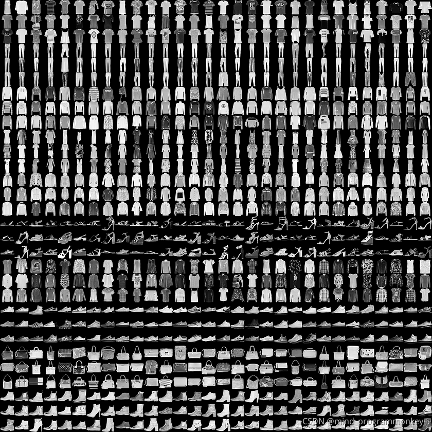
Fashion MNIST 是一个包含 70000 张灰度图像,涵盖 10 个类别(T恤,鞋子等类别)的图像数据集。以下图像显示了单件服饰在较低分辨率(28x28 像素)下的效果:
下面将做什么呢?
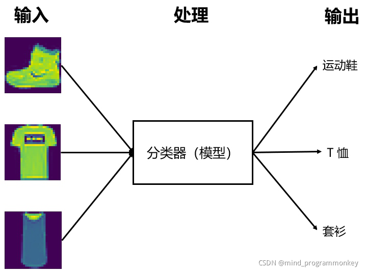
一、导入Fashion Mnist
1.导入模块
# 导入库
import tensorflow as tf
from tensorflow import keras

import numpy as np
import matplotlib.pyplot as plt
D:\software\Anaconda\anaconda\envs\tensorflow\lib\site-packages\tensorflow\python\framework\dtypes.py:516: FutureWarning: Passing (type, 1) or '1type' as a synonym of type is deprecated; in a future version of numpy, it will be understood as (type, (1,)) / '(1,)type'.
  _np_qint8 = np.dtype([("qint8", np.int8, 1)])
D:\software\Anaconda\anaconda\envs\tensorflow\lib\site-packages\tensorflow\python\framework\dtypes.py:517: FutureWarning: Passing (type, 1) or '1type' as a synonym of type is deprecated; in a future version of numpy, it will be understood as (type, (1,)) / '(1,)type'.
  _np_quint8 = np.dtype([("quint8", np.uint8, 1)])
D:\software\Anaconda\anaconda\envs\tensorflow\lib\site-packages\tensorflow\python\framework\dtypes.py:518: FutureWarning: Passing (type, 1) or '1type' as a synonym of type is deprecated; in a future version of numpy, it will be understood as (type, (1,)) / '(1,)type'.
  _np_qint16 = np.dtype([("qint16", np.int16, 1)])
D:\software\Anaconda\anaconda\envs\tensorflow\lib\site-packages\tensorflow\python\framework\dtypes.py:519: FutureWarning: Passing (type, 1) or '1type' as a synonym of type is deprecated; in a future version of numpy, it will be understood as (type, (1,)) / '(1,)type'.
  _np_quint16 = np.dtype([("quint16", np.uint16, 1)])
D:\software\Anaconda\anaconda\envs\tensorflow\lib\site-packages\tensorflow\python\framework\dtypes.py:520: FutureWarning: Passing (type, 1) or '1type' as a synonym of type is deprecated; in a future version of numpy, it will be understood as (type, (1,)) / '(1,)type'.
  _np_qint32 = np.dtype([("qint32", np.int32, 1)])
D:\software\Anaconda\anaconda\envs\tensorflow\lib\site-packages\tensorflow\python\framework\dtypes.py:525: FutureWarning: Passing (type, 1) or '1type' as a synonym of type is deprecated; in a future version of numpy, it will be understood as (type, (1,)) / '(1,)type'.
  np_resource = np.dtype([("resource", np.ubyte, 1)])
D:\software\Anaconda\anaconda\envs\tensorflow\lib\site-packages\tensorboard\compat\tensorflow_stub\dtypes.py:541: FutureWarning: Passing (type, 1) or '1type' as a synonym of type is deprecated; in a future version of numpy, it will be understood as (type, (1,)) / '(1,)type'.
  _np_qint8 = np.dtype([("qint8", np.int8, 1)])
D:\software\Anaconda\anaconda\envs\tensorflow\lib\site-packages\tensorboard\compat\tensorflow_stub\dtypes.py:542: FutureWarning: Passing (type, 1) or '1type' as a synonym of type is deprecated; in a future version of numpy, it will be understood as (type, (1,)) / '(1,)type'.
  _np_quint8 = np.dtype([("quint8", np.uint8, 1)])
D:\software\Anaconda\anaconda\envs\tensorflow\lib\site-packages\tensorboard\compat\tensorflow_stub\dtypes.py:543: FutureWarning: Passing (type, 1) or '1type' as a synonym of type is deprecated; in a future version of numpy, it will be understood as (type, (1,)) / '(1,)type'.
  _np_qint16 = np.dtype([("qint16", np.int16, 1)])
D:\software\Anaconda\anaconda\envs\tensorflow\lib\site-packages\tensorboard\compat\tensorflow_stub\dtypes.py:544: FutureWarning: Passing (type, 1) or '1type' as a synonym of type is deprecated; in a future version of numpy, it will be understood as (type, (1,)) / '(1,)type'.
  _np_quint16 = np.dtype([("quint16", np.uint16, 1)])
D:\software\Anaconda\anaconda\envs\tensorflow\lib\site-packages\tensorboard\compat\tensorflow_stub\dtypes.py:545: FutureWarning: Passing (type, 1) or '1type' as a synonym of type is deprecated; in a future version of numpy, it will be understood as (type, (1,)) / '(1,)type'.
  _np_qint32 = np.dtype([("qint32", np.int32, 1)])
D:\software\Anaconda\anaconda\envs\tensorflow\lib\site-packages\tensorboard\compat\tensorflow_stub\dtypes.py:550: FutureWarning: Passing (type, 1) or '1type' as a synonym of type is deprecated; in a future version of numpy, it will be understood as (type, (1,)) / '(1,)type'.
  np_resource = np.dtype([("resource", np.ubyte, 1)])
在tf.keras中已经集成了下载与加载Fashion-MNIST数据集的骨架程序,只需要导入与加载数据即可,数据集中的60000图片用于训练网络,10000张图片用于评估经过学习的网络分类图像的准确率
注:在机器学习中,我们一般会将数据集按照8:2的比例分为训练数据集和测试数据集,训练数据集用于训练模型,测试数据集用于测试训练好的模型的准确率.
2.加载数据集
# 加载数据集
fashion_mnist = keras.datasets.fashion_mnist

(train_images, train_labels), (test_images, test_labels) = fashion_mnist.load_data()
加载完数据集后会返回4个 Numpy 数组
- train_images 和 train_labels 数组是训练集,即模型用于学习的数据,共有60000张
- 测试集 test_images 和 test_labels 数组用于测试模型。共有10000张
- train_images 和 test_images 中都为 28x28 的 NumPy 数组,每个点的值都是介于 0 到 255 之间。代表了当前这张图片 test_images 和test_labels是一个10维的整数数组,每个维度的值都是介于0到9之间。代表了当前图像的标签,这些标签对应于图像代表的服饰所属的类别:
3.探索数据集
#我们先探索数据集的格式,然后再训练模型。我们先查看一下数据集中的图片的形状
print(train_images.shape)
(60000, 28, 28)
#我们再查看一下 数据集中标签的形状
print(train_labels.shape)
(60000,)
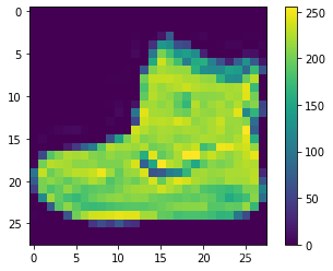
# 可视化
## 创建新的图像
plt.figure()
## 显示图像 (填入图像)
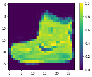
plt.imshow(train_images[0])
## 给子图添加colorbar(颜色条或渐变色条)
plt.colorbar()
## 设置网格线
plt.grid(False)
4.查看标签
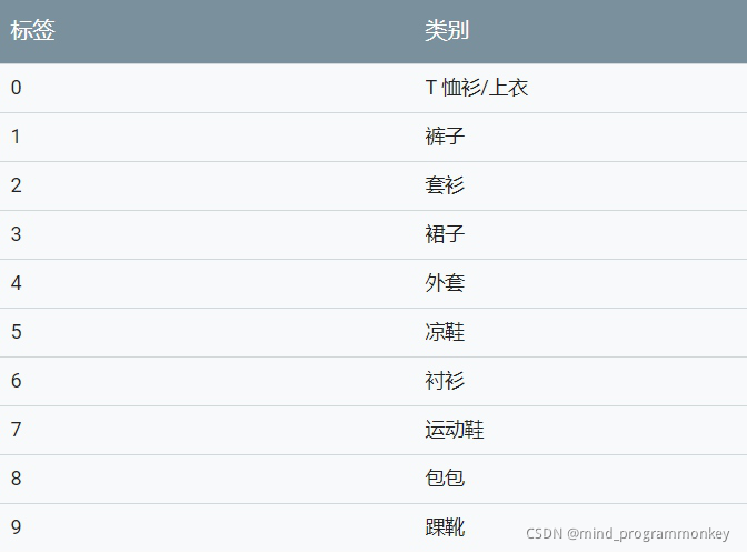
class_names = ['T-shirt/top', 'Trouser', 'Pullover', 'Dress', 'Coat',
               'Sandal', 'Shirt', 'Sneaker', 'Bag', 'Ankle boot']
print(train_labels[0])
print(class_names[train_labels[0]])
9
Ankle boot
5.预处理归一化操作
我们将图片中的这些值缩小到 0 到 1 之间,然后将其馈送到神经网络模型。为此,将图像组件的数据类型从整数转换为浮点数,然后除以 255。这样更容易训练,以下是预处理图像的函数:务必要以相同的方式对训练集和测试集进行预处理:
train_images = train_images / 255.0
test_images = test_images / 255.0
# 显示预处理完之后的图像
plt.figure()
plt.imshow(train_images[0])
plt.colorbar()
plt.grid(False)
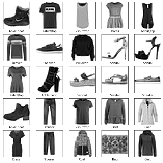
#显示训练集中的前 25 张图像,并在每张图像下显示类别名称。验证确保数据格式正确无误,然后我们就可以开始构建和训练网络了。
plt.figure(figsize=(10,10))
for i in range(25):
    ## 在当前图下生成子图 5*5个图
    plt.subplot(5,5,i+1)
    plt.xticks([])
    plt.yticks([])
    plt.grid(False)
    plt.imshow(train_images[i], cmap=plt.cm.binary)
    #显示 当前图片的类别
    plt.xlabel(class_names[train_labels[i]])
二、基于词袋模型
- (1)依然是对每张图片提取其特征点,比如提取了SIFT特征点
- (2)对所有图片的所有的SIFT特征点,整体进行kmeans聚类,将词划分成多个不同的类,类的个数定义为wordCount。
- (3)对每张图片,计算不同的类的SIFT特征的个数,对应所要得到的特征向量中的一个维度。则我们可以对每张图片生成一个wordCount维的向量。
取得一幅图像的BoW向量的步骤:
- 构建图像库的视觉词典Vocabulary
- 提取图像库中所有图像的局部特征,如SIFT.
- 对提取到的图像特征进行聚类,如k-means,得到聚类中心就是图像库的视觉词汇词典Vocabulary
- 计算一幅图像的BoW向量
- 提取图像的局部特征
- 统计Vocabulay中的每个视觉词汇visual word ,在图像中出现的频率。
import os
import cv2
import pickle
import numpy as np
import matplotlib.pyplot as plt
from imutils import paths
from sklearn.cluster import KMeans
from scipy.cluster.vq import vq
from sklearn.model_selection import train_test_split

from sklearn.svm import LinearSVC
print(train_images.shape)
print(train_labels.shape)
print(test_images.shape)
print(test_labels.shape)
(60000, 28, 28)
(60000,)
(10000, 28, 28)
(10000,)
sifts_img = [] # 存放所有图像的文件名和sift特征

limit = 10000 #最大训练个数

count = 0 # 词袋特征个数
num = 0 # 有效个数
label = []
for i in range(limit):
    img = train_images[i].reshape(28,28)
    img = np.uint8(np.double(img) * 255)
    sift = cv2.xfeatures2d.SIFT_create()
    kp,des = sift.detectAndCompute(img,None)
    if des is None:
        continue
    sifts_img.append(des)
    label.append(train_labels[i])
    count = count + des.shape[0]
    num = num + 1

label = np.array(label)

data = sifts_img[0]
for des in sifts_img[1:]:
    data = np.vstack((data, des))

print("train file:",num)
count = int(count / 40)
count = max(4,count)
train file: 9236
# 对sift特征进行聚类
k_means = KMeans(n_clusters=int(count), n_init=4)
k_means.fit(data)


# 构建所有样本的词袋表示
image_features = np.zeros([int(num),int(count)],'float32')
for i in range(int(num)):
    ws, d = vq(sifts_img[i],k_means.cluster_centers_)# 计算各个sift特征所属的视觉词汇
    for w in ws:
        image_features[i][w] += 1  # 对应视觉词汇位置元素加1


x_tra, x_val, y_tra, y_val = train_test_split(image_features,label,test_size=0.2)
# 构建线性SVM对象并训练
clf = LinearSVC(C=1, loss="hinge").fit(x_tra, y_tra)
# 训练数据预测正确率
print (clf.score(x_val, y_val))


# save the training model as pickle
with open('bow_kmeans.pickle','wb') as fw:
    pickle.dump(k_means,fw)
with open('bow_clf.pickle','wb') as fw:
    pickle.dump(clf,fw)
with open('bow_count.pickle','wb') as fw:
    pickle.dump(count,fw)
print('Trainning successfully and save the model')
0.6293290043290043
Trainning successfully and save the model


D:\software\Anaconda\anaconda\envs\tensorflow\lib\site-packages\sklearn\svm\_base.py:947: ConvergenceWarning: Liblinear failed to converge, increase the number of iterations.
  "the number of iterations.", ConvergenceWarning)
with open('bow_kmeans.pickle','rb') as fr:
    k_means = pickle.load(fr)
with open('bow_clf.pickle','rb') as fr:
    clf = pickle.load(fr)
with open('bow_count.pickle','rb') as fr:
    count = pickle.load(fr)

target_file = ['T-shirt','Trouser','Pullover',
               'Dress','Coat','Sandal','Shirt',
               'Sneaker','Bag','Ankle boot']

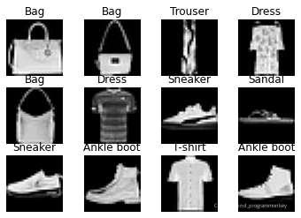
plt.figure()
cnt = 30
i = 1
while(i<=12):
    img = test_images[cnt].reshape(28,28)
    cnt = cnt + 1
    img = np.uint8(np.double(img) * 255)
    sift = cv2.xfeatures2d.SIFT_create()
    kp,des = sift.detectAndCompute(img,None)
    if des is None:
        continue
    words, distance = vq(des, k_means.cluster_centers_)
    image_features_search = np.zeros((int(count)), "float32")
    for w in words:
        image_features_search[w] += 1
    t = clf.predict(image_features_search.reshape(1,-1))
    plt.subplot(3,4,i)
    i += 1
    plt.imshow(img,'gray')
    plt.title(target_file[t[0]])
    plt.axis('off')
plt.show()
with open('bow_kmeans.pickle','rb') as fr:
    k_means = pickle.load(fr)
with open('bow_clf.pickle','rb') as fr:
    clf = pickle.load(fr)
with open('bow_count.pickle','rb') as fr:
    count = pickle.load(fr)


i = 0
len = test_images.shape[0]
predict_arr = []

while(i<len):
    img = test_images[i].reshape(28,28)
    img = np.uint8(np.double(img) * 255)
    sift = cv2.xfeatures2d.SIFT_create()
    print(i)
    kp,des = sift.detectAndCompute(img,None)
    if des is None:
        i += 1
        predict_arr.append(0)
        continue
    words, distance = vq(des, k_means.cluster_centers_)
    image_features_search = np.zeros((int(count)), "float32")
    for w in words:
        image_features_search[w] += 1
    t = clf.predict(image_features_search.reshape(1,-1))
    i += 1
    predict_arr.append(t[0])
0
1
2
3
4
5
6
7
8
9
10
11
12
13
14
15
16
17
18
19
20
21
22
23
24
25
26
27
28
29
30
31
32
33
34
35


9995
9996
9997
9998
9999
from sklearn.metrics import accuracy_score,f1_score,confusion_matrix,classification_report

score=accuracy_score(test_labels,predict_arr)
print(score)
0.5651
print(classification_report(test_labels,predict_arr))
              precision    recall  f1-score   support

           0       0.36      0.60      0.45      1000
           1       0.72      0.47      0.57      1000
           2       0.43      0.47      0.45      1000
           3       0.49      0.46      0.47      1000
           4       0.45      0.44      0.44      1000
           5       0.79      0.74      0.76      1000
           6       0.36      0.24      0.29      1000
           7       0.74      0.74      0.74      1000
           8       0.67      0.66      0.66      1000
           9       0.79      0.84      0.81      1000

    accuracy                           0.57     10000
   macro avg       0.58      0.57      0.56     10000
weighted avg       0.58      0.57      0.56     10000
import seaborn as sns
from sklearn.metrics import confusion_matrix
import matplotlib.pyplot as plt
%matplotlib inline
sns.set()

# 混淆矩阵


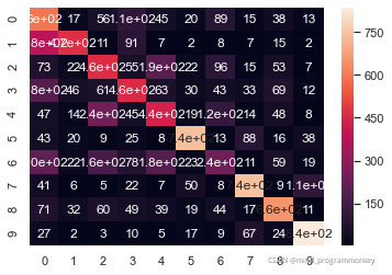
matrix = confusion_matrix(test_labels,predict_arr)
print(matrix)
sns.heatmap(matrix,annot=True)
[[598  17  56 109  45  20  89  15  38  13]
 [384 473  11  91   7   2   8   7  15   2]
 [ 73  22 465  55 192  22  96  15  53   7]
 [184  46  61 459  63  30  43  33  69  12]
 [ 47  14 245  45 441  19 119  14  48   8]
 [ 43  20   9  25   8 740  13  88  16  38]
 [205  22 161  78 184  23 238  11  59  19]
 [ 41   6   5  22   7  50   8 743   9 109]
 [ 71  32  60  49  39  19  44  17 658  11]
 [ 27   2   3  10   5  17   9  67  24 836]]


<matplotlib.axes._subplots.AxesSubplot at 0x1f384714548>
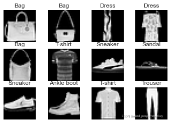
三、基于HOG特征
Histogram of Oriented Gridients,缩写为HOG,是目前计算机视觉、模式识别领域很常用的一种描述图像局部纹理的特征。这个特征名字起的也很直白,就是说先计算图片某一区域中不同方向上梯度的值,然后进行累积,得到直方图,这个直方图呢,就可以代表这块区域了,也就是作为特征,可以输入到分类器里面了。那么,接下来介绍一下HOG的具体原理和计算方法,以及一些引申。
因为HOG是一个局部特征,因此如果你对一大幅图片直接提取特征,是得不到好的效果的。原理很简单。从信息论角度讲,例如一幅640*480的图像,大概有30万个像素点,也就是说原始数据有30万维特征,如果直接做HOG的话,就算按照360度,分成360个bin,也没有表示这么大一幅图像的能力。从特征工程的角度看,一般来说,只有图像区域比较小的情况,基于统计原理的直方图对于该区域才有表达能力,如果图像区域比较大,那么两个完全不同的图像的HOG特征,也可能很相似。但是如果区域较小,这种可能性就很小。最后,把图像分割成很多区块,然后对每个区块计算HOG特征,这也包含了几何(位置)特性。例如,正面的人脸,左上部分的图像区块提取的HOG特征一般是和眼睛的HOG特征符合的。
import warnings
warnings.filterwarnings("ignore")

import os
import cv2
import pickle
import numpy as np
import matplotlib.pyplot as plt
from imutils import paths
from skimage.feature import hog
from scipy.cluster.vq import vq
from sklearn.svm import LinearSVC
from sklearn.model_selection import train_test_split
limit = train_images.shape[0]

data = [] # HoG特征
label = []
for i in range(limit):
    img = train_images[i].reshape(28,28)
    img = np.uint8(np.double(img) * 255)
    fd = hog(img)
    data.append(fd)
    label.append(train_labels[i])

data = np.array(data)
label = np.array(label)

x_tra, x_val, y_tra, y_val = train_test_split(data,label,test_size=0.2)

print('train file:',y_tra.size)
print('val file:',y_val.size)

# 构建线性SVM对象并训练
clf = LinearSVC(C=1, loss="hinge").fit(x_tra, y_tra)
# 训练数据预测正确率
print ('accuracy:',clf.score(x_val, y_val))


# save the training model as pickle
with open('hog.pickle','wb') as fw:
    pickle.dump(clf,fw)
print('Trainning successfully and save the model')
train file: 48000
val file: 12000
accuracy: 0.799
Trainning successfully and save the model
with open('hog.pickle','rb') as fr:
    clf = pickle.load(fr)

target_file = ['T-shirt','Trouser','Pullover',
               'Dress','Coat','Sandal','Shirt',
               'Sneaker','Bag','Ankle boot']

plt.figure()
cnt = 30
i = 1
while(i<=12):
    img = test_images[cnt].reshape(28,28)
    cnt = cnt + 1
    img = np.uint8(np.double(img) * 255)
    fd = hog(img)
    t = clf.predict([fd])
    plt.subplot(3,4,i)
    i += 1
    plt.imshow(img,'gray')
    plt.title(target_file[t[0]])
    plt.axis('off')
plt.show()
with open('hog.pickle','rb') as fr:
    clf = pickle.load(fr)


i = 0
len = test_images.shape[0]
predict_arr = []

while(i<len):
    img = test_images[i].reshape(28,28)
    img = np.uint8(np.double(img) * 255)
    fd = hog(img)
    t = clf.predict([fd])
    i += 1
    predict_arr.append(t[0])
from sklearn.metrics import accuracy_score,f1_score,confusion_matrix,classification_report

score=accuracy_score(test_labels,predict_arr)
print(score)
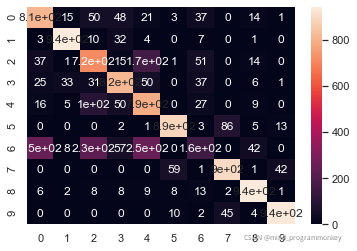
0.7904
print(classification_report(test_labels,predict_arr))
              precision    recall  f1-score   support

           0       0.70      0.81      0.75      1000
           1       0.94      0.94      0.94      1000
           2       0.62      0.71      0.67      1000
           3       0.79      0.82      0.81      1000
           4       0.61      0.79      0.69      1000
           5       0.92      0.89      0.90      1000
           6       0.47      0.16      0.24      1000
           7       0.87      0.90      0.88      1000
           8       0.91      0.94      0.92      1000
           9       0.94      0.94      0.94      1000

    accuracy                           0.79     10000
   macro avg       0.78      0.79      0.77     10000
weighted avg       0.78      0.79      0.77     10000
import seaborn as sns
from sklearn.metrics import confusion_matrix
import matplotlib.pyplot as plt
%matplotlib inline
sns.set()

# 混淆矩阵


matrix = confusion_matrix(test_labels,predict_arr)
print(matrix)
sns.heatmap(matrix,annot=True)
[[811  15  50  48  21   3  37   0  14   1]
 [  3 943  10  32   4   0   7   0   1   0]
 [ 37   1 715  15 166   1  51   0  14   0]
 [ 25  33  31 817  50   0  37   0   6   1]
 [ 16   5 103  50 790   0  27   0   9   0]
 [  0   0   0   2   1 890   3  86   5  13]
 [253   8 228  57 253   0 159   0  42   0]
 [  0   0   0   0   0  59   1 897   1  42]
 [  6   2   8   8   9   8  13   2 943   1]
 [  0   0   0   0   0  10   2  45   4 939]]


<matplotlib.axes._subplots.AxesSubplot at 0x1f382c92408>
四、MLP多层感知器
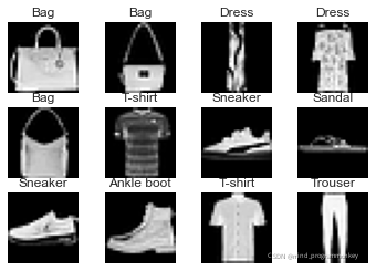
多层感知机(MLP,Multilayer Perceptron)也叫人工神经网络(ANN,Artificial Neural Network),除了输入输出层,它中间可以有多个隐层,最简单的MLP只含一个隐层,即三层的结构
import numpy as np
from keras.models import Sequential
from keras.layers import Dense, Dropout, Flatten, Activation
from keras.layers import Conv2D, MaxPooling2D
from keras.utils.vis_utils import plot_model
from keras.utils import np_utils
X_train = train_images.reshape((-1,784))
X_test = test_images.reshape(-1,784)
Y_train = np_utils.to_categorical(train_labels,num_classes=10)
Y_test = np_utils.to_categorical(test_labels,num_classes=10)
# Build MLP
model = Sequential()

model.add(Dense(units=256,
                input_dim=784,
                kernel_initializer='normal',
                activation='relu'))

model.add(Dense(units=10,
                kernel_initializer='normal',
                activation='softmax'))

model.summary()
_________________________________________________________________
Layer (type)                 Output Shape              Param #
=================================================================
dense_3 (Dense)              (None, 256)               200960
_________________________________________________________________
dense_4 (Dense)              (None, 10)                2570
=================================================================
Total params: 203,530
Trainable params: 203,530
Non-trainable params: 0
_________________________________________________________________
model.compile(loss='categorical_crossentropy', optimizer='adam', metrics=['accuracy'])
model.fit(X_train, Y_train, batch_size=500, epochs=10, verbose=1, validation_data=(X_test, Y_test))
model.save('mlp_fashion_mnist.h5')
WARNING:tensorflow:From D:\software\Anaconda\anaconda\envs\tensorflow\lib\site-packages\tensorflow\python\ops\math_grad.py:1250: add_dispatch_support.<locals>.wrapper (from tensorflow.python.ops.array_ops) is deprecated and will be removed in a future version.
Instructions for updating:
Use tf.where in 2.0, which has the same broadcast rule as np.where
WARNING:tensorflow:From D:\software\Anaconda\anaconda\envs\tensorflow\lib\site-packages\keras\backend\tensorflow_backend.py:977: The name tf.assign_add is deprecated. Please use tf.compat.v1.assign_add instead.

Train on 60000 samples, validate on 10000 samples
Epoch 1/10
60000/60000 [==============================] - 28s 459us/step - loss: 0.6751 - acc: 0.7771 - val_loss: 0.4986 - val_acc: 0.8310
Epoch 2/10
60000/60000 [==============================] - 1s 19us/step - loss: 0.4437 - acc: 0.8480 - val_loss: 0.4469 - val_acc: 0.8400
Epoch 3/10
60000/60000 [==============================] - 2s 31us/step - loss: 0.3997 - acc: 0.8609 - val_loss: 0.4300 - val_acc: 0.8481
Epoch 4/10
60000/60000 [==============================] - 1s 18us/step - loss: 0.3749 - acc: 0.8682 - val_loss: 0.4151 - val_acc: 0.8546
Epoch 5/10
60000/60000 [==============================] - 1s 18us/step - loss: 0.3512 - acc: 0.8767 - val_loss: 0.3819 - val_acc: 0.8646
Epoch 6/10
60000/60000 [==============================] - 1s 19us/step - loss: 0.3345 - acc: 0.8819 - val_loss: 0.3882 - val_acc: 0.8625
Epoch 7/10
60000/60000 [==============================] - 1s 19us/step - loss: 0.3224 - acc: 0.8855 - val_loss: 0.3654 - val_acc: 0.8725
Epoch 8/10
60000/60000 [==============================] - 1s 19us/step - loss: 0.3086 - acc: 0.8889 - val_loss: 0.3558 - val_acc: 0.8723
Epoch 9/10
60000/60000 [==============================] - 1s 18us/step - loss: 0.2980 - acc: 0.8926 - val_loss: 0.3548 - val_acc: 0.8744
Epoch 10/10
60000/60000 [==============================] - 1s 19us/step - loss: 0.2879 - acc: 0.8963 - val_loss: 0.3560 - val_acc: 0.8719
from keras.models import load_model
model = load_model('mlp_fashion_mnist.h5')
plt.figure()
cnt = 30
i = 1
while(i<=12):
    img = [X_test[cnt]]
    cnt = cnt + 1
    img = np.uint8(np.double(img) * 255)
    t = model.predict(img)
    result = np.argmax(t, axis=1)
    plt.subplot(3,4,i)
    i += 1
    plt.imshow(img[0].reshape(28,28),'gray')
    plt.title(target_file[result[0]])
    plt.axis('off')
plt.show()
loss, accuracy = model.evaluate(X_test, Y_test, verbose=0)
print('loss:', loss)
print('accuracy:', accuracy)
loss: 0.35601275362968443
accuracy: 0.8719
predict = model.predict_classes(X_test)

from sklearn.metrics import accuracy_score,f1_score,confusion_matrix,classification_report

score=accuracy_score(test_labels,predict)
print(score)
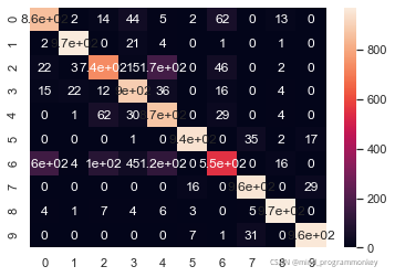
0.8719
print(classification_report(test_labels,predict))
              precision    recall  f1-score   support

           0       0.81      0.86      0.83      1000
           1       0.97      0.97      0.97      1000
           2       0.79      0.74      0.76      1000
           3       0.85      0.90      0.87      1000
           4       0.72      0.87      0.79      1000
           5       0.97      0.94      0.96      1000
           6       0.78      0.55      0.65      1000
           7       0.93      0.95      0.94      1000
           8       0.96      0.97      0.96      1000
           9       0.95      0.96      0.96      1000

    accuracy                           0.87     10000
   macro avg       0.87      0.87      0.87     10000
weighted avg       0.87      0.87      0.87     10000
import seaborn as sns
from sklearn.metrics import confusion_matrix
import matplotlib.pyplot as plt
%matplotlib inline
sns.set()

# 混淆矩阵


matrix = confusion_matrix(test_labels,predict)
print(matrix)
sns.heatmap(matrix,annot=True)
[[858   2  14  44   5   2  62   0  13   0]
 [  2 971   0  21   4   0   1   0   1   0]
 [ 22   3 739  15 173   0  46   0   2   0]
 [ 15  22  12 895  36   0  16   0   4   0]
 [  0   1  62  30 874   0  29   0   4   0]
 [  0   0   0   1   0 945   0  35   2  17]
 [161   4 100  45 123   0 551   0  16   0]
 [  0   0   0   0   0  16   0 955   0  29]
 [  4   1   7   4   6   3   0   5 970   0]
 [  0   0   0   0   0   7   1  31   0 961]]


<matplotlib.axes._subplots.AxesSubplot at 0x1f383b67a48>
五、CNN卷积神经网络
import numpy as np
from keras.models import Sequential
from keras.layers import Dense, Dropout, Flatten, Activation
from keras.layers import Conv2D, MaxPooling2D
from keras.utils.vis_utils import plot_model
from keras.utils import np_utils
X_train = train_images.reshape((-1,28,28,1))
X_test = test_images.reshape(-1,28,28,1)
Y_train = np_utils.to_categorical(train_labels,num_classes=10)
Y_test = np_utils.to_categorical(test_labels,num_classes=10)
# Build LeNet-5
model = Sequential()
model.add(Conv2D(filters=6, kernel_size=(5, 5), padding='valid', input_shape=(28, 28, 1), activation='relu')) # C1
model.add(MaxPooling2D(pool_size=(2, 2))) # S2
model.add(Conv2D(filters=16, kernel_size=(5, 5), padding='valid', activation='relu')) # C3
model.add(MaxPooling2D(pool_size=(2, 2))) # S4
model.add(Flatten())
model.add(Dense(120, activation='tanh')) # C5
model.add(Dense(84, activation='tanh')) # F6
model.add(Dense(10, activation='softmax')) # output
model.summary()
_________________________________________________________________
Layer (type)                 Output Shape              Param #
=================================================================
conv2d_3 (Conv2D)            (None, 24, 24, 6)         156
_________________________________________________________________
max_pooling2d_3 (MaxPooling2 (None, 12, 12, 6)         0
_________________________________________________________________
conv2d_4 (Conv2D)            (None, 8, 8, 16)          2416
_________________________________________________________________
max_pooling2d_4 (MaxPooling2 (None, 4, 4, 16)          0
_________________________________________________________________
flatten_2 (Flatten)          (None, 256)               0
_________________________________________________________________
dense_8 (Dense)              (None, 120)               30840
_________________________________________________________________
dense_9 (Dense)              (None, 84)                10164
_________________________________________________________________
dense_10 (Dense)             (None, 10)                850
=================================================================
Total params: 44,426
Trainable params: 44,426
Non-trainable params: 0
_________________________________________________________________
model.compile(loss='categorical_crossentropy', optimizer='adam', metrics=['accuracy'])
model.fit(X_train, Y_train, batch_size=500, epochs=10, verbose=1, validation_data=(X_test, Y_test))
model.save('cnn_fashion_mnist.h5')
Train on 60000 samples, validate on 10000 samples
Epoch 1/10
60000/60000 [==============================] - 3s 44us/step - loss: 0.3044 - acc: 0.8892 - val_loss: 0.3304 - val_acc: 0.8774
Epoch 2/10
60000/60000 [==============================] - 2s 34us/step - loss: 0.2902 - acc: 0.8948 - val_loss: 0.3259 - val_acc: 0.8809
Epoch 3/10
60000/60000 [==============================] - 2s 35us/step - loss: 0.2826 - acc: 0.8967 - val_loss: 0.3145 - val_acc: 0.8865
Epoch 4/10
60000/60000 [==============================] - 2s 33us/step - loss: 0.2724 - acc: 0.9002 - val_loss: 0.3158 - val_acc: 0.8862
Epoch 5/10
60000/60000 [==============================] - 2s 33us/step - loss: 0.2683 - acc: 0.9025 - val_loss: 0.3174 - val_acc: 0.8843
Epoch 6/10
60000/60000 [==============================] - 2s 34us/step - loss: 0.2610 - acc: 0.9047 - val_loss: 0.3040 - val_acc: 0.8900
Epoch 7/10
60000/60000 [==============================] - 2s 34us/step - loss: 0.2519 - acc: 0.9082 - val_loss: 0.3015 - val_acc: 0.8904
Epoch 8/10
60000/60000 [==============================] - 2s 33us/step - loss: 0.2481 - acc: 0.9086 - val_loss: 0.3097 - val_acc: 0.8877
Epoch 9/10
60000/60000 [==============================] - 2s 34us/step - loss: 0.2432 - acc: 0.9107 - val_loss: 0.2940 - val_acc: 0.8936
Epoch 10/10
60000/60000 [==============================] - 2s 34us/step - loss: 0.2355 - acc: 0.9134 - val_loss: 0.2934 - val_acc: 0.8924
loss, accuracy = model.evaluate(X_test, Y_test, verbose=0)
print('loss:', loss)
print('accuracy:', accuracy)
loss: 0.29342212826013564
accuracy: 0.8924
predict = model.predict_classes(X_test)

from sklearn.metrics import accuracy_score,f1_score,confusion_matrix,classification_report

score=accuracy_score(test_labels,predict)
print(score)
0.8924
print(classification_report(test_labels,predict))
              precision    recall  f1-score   support

           0       0.80      0.88      0.84      1000
           1       0.99      0.97      0.98      1000
           2       0.81      0.87      0.84      1000
           3       0.88      0.91      0.90      1000
           4       0.83      0.82      0.83      1000
           5       0.97      0.97      0.97      1000
           6       0.75      0.62      0.68      1000
           7       0.92      0.97      0.95      1000
           8       0.97      0.98      0.97      1000
           9       0.98      0.94      0.96      1000

    accuracy                           0.89     10000
   macro avg       0.89      0.89      0.89     10000
weighted avg       0.89      0.89      0.89     10000
import seaborn as sns
from sklearn.metrics import confusion_matrix
import matplotlib.pyplot as plt
%matplotlib inline
sns.set()

# 混淆矩阵


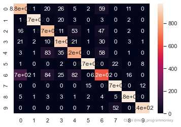
matrix = confusion_matrix(test_labels,predict)
print(matrix)
sns.heatmap(matrix,annot=True)
[[876   1  20  26   5   2  59   0  11   0]
 [  1 971   0  20   3   0   3   0   2   0]
 [ 16   1 869  11  53   1  47   0   2   0]
 [ 21   2  10 911  21   1  30   0   3   1]
 [  3   1  83  35 819   0  58   0   1   0]
 [  1   0   0   2   0 967   0  22   0   8]
 [170   1  84  25  82   0 622   0  16   0]
 [  0   0   0   0   0  15   0 973   0  12]
 [  5   1   3   3   1   2   4   5 976   0]
 [  0   0   0   0   0   7   1  52   0 940]]


<matplotlib.axes._subplots.AxesSubplot at 0x1f4444938c8>
小结
那么本次实验就到此结束,点赞评论收藏一条龙走起来,瓷们!!!!

 1万+


 扫一扫


 被折叠的 条评论
为什么被折叠?
 到【灌水乐园】发言


