#GEE
library(multgee)
library(dplyr)
library(stringr)
library(openxlsx)
df_long2 <- df_long %>%
# 受试者ID列名请替换成你真实的,比如 bian_hao;这里假设叫 bian_hao
rename(id = bian_hao) %>%
filter(!is.na(StoolType)) %>%
mutate(
group = factor(group, levels = c("3","6","1")), # 3 为参照组
StoolType = ordered(StoolType), # 确保有序
Timepoint = factor(Timepoint, ordered = TRUE) # 确保 V0 是第一层
)
df_long2 <- df_long2 %>%
mutate(
age_days_V0_z = scale(age_days_V0),
mu_qin_yunqian_bmi_V0_z = scale(mu_qin_yunqian_bmi_V0),
yunzhou_V0_z = scale(yunzhou_V0),
chu_sheng_ti_zhong_V0_z = scale(chu_sheng_ti_zhong_V0)
)
df_long2 <- df_long2 %>% mutate(
Timepoint = factor(Timepoint, ordered = FALSE) # 取消有序
)
contrasts(df_long2$Timepoint) <- contr.treatment(levels(df_long2$Timepoint)) # 以 V0 为参照
# ========= 2) 拟合有序 GEE 模型(cumulative logit)=========
# LORstr 可选 "uniform", "category.exch";repeated 指定时间变量
fit_ordgee <- ordLORgee(
formula = StoolType ~ group * Timepoint +
age_days_V0_z + xing_bie_V0 + chu_sheng_ti_zhong_V0_z +
fen_mian_fang_shi_V0 + region +
mu_qin_yunqian_bmi_V0_z + yunzhou_V0_z + income_cat +
muqin_education_V0,
id = id,
repeated = Timepoint,
data = df_long2,
link = "logit",
LORstr = "uniform",
add = 0.5 # 防止某些格为0导致估计不稳定
)
summary(fit_ordgee)
#三组间整体检验
## 1) 从模型中取系数 & 协方差,并确保 b 有名字
s <- summary(fit_ordgee)
b <- as.numeric(s$coef[, "Estimate"])
names(b) <- rownames(s$coef) # 关键:给 b 加上行名作为 names
V <- if (!is.null(fit_ordgee$robust.variance)) fit_ordgee$robust.variance else vcov(fit_ordgee)
coef_names <- names(b)
print(coef_names) # 看看真实行名长啥样
## 2) 通用的整体 Wald 检验函数(无任何外部包)
wald_overall <- function(b, V, terms){
idx <- match(terms, names(b))
idx <- idx[!is.na(idx)]
if (length(idx) == 0) stop("没有匹配到参数名")
R <- diag(length(b))[idx, , drop = FALSE]
rb <- R %*% b
RVRT <- R %*% V %*% t(R)
W <- as.numeric(t(rb) %*% solve(RVRT) %*% rb)
df <- length(idx)
p <- 1 - pchisq(W, df)
data.frame(chi2 = W, df = df, p = p, row.names = NULL)
}
## 3) 通用匹配规则(不假设“=”或“.”,也兼容 Time 与 Timepoint)
## - 组主效应:以 "group" 开头,且不含 ":"(不是交互项)
terms_group_main <- coef_names[ grepl("^group", coef_names) & !grepl(":", coef_names) ]
## - 时间主效应:以 "Time" 或 "Timepoint" 开头,且不含 ":"(不是交互)
terms_time_main <- coef_names[ grepl("^(Time|Timepoint)", coef_names) & !grepl(":", coef_names) ]
## - 组×时间交互:以 "group" 开头,且后面有 ":",并且冒号后面跟的是 Time/Timepoint
terms_gxt <- coef_names[ grepl("^group", coef_names) & grepl(":(Time|Timepoint)", coef_names) ]
## 4) 跑整体检验
cat("== Group 主效应 ==\n"); print(wald_overall(b, V, terms_group_main))
cat("== Time 主效应 ==\n"); print(wald_overall(b, V, terms_time_main))
cat("== Group × Time 交互 ==\n"); print(wald_overall(b, V, terms_gxt))
#整体间交互项有显著性差异
# 注意:系数是 log(累积OR),exp() 后就是 累积OR
# ========= 3) 提取系数,换算为 OR + 95%CI + P =========
coef_tab <- summary(fit_ordgee)$coef
# 计算95%CI(β和OR双尺度),保留更多小数
beta_CI_low <- coef_tab[, "Estimate"] - qnorm(0.975) * coef_tab[, "san.se"]
beta_CI_high <- coef_tab[, "Estimate"] + qnorm(0.975) * coef_tab[, "san.se"]
out_coef <- data.frame(
term = rownames(coef_tab),
beta = round(coef_tab[, "Estimate"], 6),
se = round(coef_tab[, "san.se"], 6),
z = round(coef_tab[, "san.z"], 6),
p_value = signif(coef_tab[, "Pr(>|san.z|)"], 6),
# beta 尺度的置信区间
beta_CI_low = round(beta_CI_low, 6),
beta_CI_high = round(beta_CI_high, 6),
# OR 尺度
OR = round(exp(coef_tab[, "Estimate"]), 6),
CI_low = round(exp(beta_CI_low), 6),
CI_high = round(exp(beta_CI_high), 6)
) %>%
mutate(
term = str_replace_all(term, "group", "group="),
term = str_replace_all(term, "Timepoint", "Time="),
term = str_replace_all(term, ":", " × ")
)
# 查看结果
print(out_coef)
# 保存总体系数表(主效应 + 交互项)
write.xlsx(out_coef, "gee_ordinal_overall_coefficients_调整协变量.xlsx", rowNames = FALSE)
#与上面的两两每时点比较类似: 更严谨的线性组合(含协方差)做两两每时点的组间比较——
lincom_cov <- function(model, L_named){
s <- summary(model)
b <- s$coef[, "Estimate"]; V <- if (!is.null(model$robust.variance)) model$robust.variance else vcov(model)
L <- rep(0, length(b)); names(L) <- rownames(s$coef)
hit <- intersect(names(L_named), names(L)); L[hit] <- L_named[hit]
est <- sum(L * b)
se <- sqrt(as.numeric(t(L) %*% V %*% L))
OR <- exp(est); CI <- exp(c(est - 1.96*se, est + 1.96*se))
z <- est / se; p <- 2*pnorm(-abs(z))
c(beta=est, se=se, OR=OR, CI_low=CI[1], CI_high=CI[2], z=z, p_value=p)
}
# —— 构造“组A vs 组B @ 指定时间点”的对比向量 ——
# 记号:A/B ∈ c("1","3","6");tp ∈ levels(df_long2$Timepoint)(如 "V0","V1",...)
# 规则:A_vs_B(tp) = [ groupA + groupA:Time_tp ] - [ groupB + groupB:Time_tp ]
build_contrast <- function(A, B, tp, coef_names){
# 主效应名(可能不存在:如果该组恰好是 group 的参照,则主效应=0)
gA <- paste0("group", A); gB <- paste0("group", B)
# 交互项名(在 treatment 对比下应是 "groupX:TimepointVt" 这种)
iA <- paste0("group", A, ":Timepoint", tp)
iB <- paste0("group", B, ":Timepoint", tp)
# 只对存在于模型的项赋值(不存在的等于0)
pick <- function(nm) nm[nm %in% coef_names]
setNames(c(rep(1, length(pick(c(gA,iA)))), rep(-1, length(pick(c(gB,iB))))),
c(pick(c(gA,iA)), pick(c(gB,iB))))
}
# —— 批量生成“三组两两 × 各时间点”的结果表 ——
pairwise_by_time <- function(model, data, timevar = "Timepoint", groups = c("1","3","6")){
coef_names <- rownames(summary(model)$coef)
tps <- levels(data[[timevar]])
out <- list()
for(tp in tps){
for(i in 1:(length(groups)-1)){
for(j in (i+1):length(groups)){
A <- groups[i]; B <- groups[j]
L <- build_contrast(A, B, tp, coef_names)
res <- lincom_cov(model, L)
out[[paste(tp, paste0(A," vs ",B), sep=" | ")]] <-
data.frame(time=tp, contrast=paste0(A," vs ",B),
t(res))
}
}
}
dplyr::bind_rows(out)
}
# 然后这样运行:
pw_tab <- pairwise_by_time(fit_ordgee, data = df_long2, timevar = "Timepoint", groups = c("1","3","6"))
pw_tab
# 保存“各时间点简单效应OR”表
write.xlsx(pw_tab, "gee_ordinal_simple_effects_by_time.xlsx", rowNames = FALSE)
#随时间点变化的两两比较
library(emmeans)
library(geepack)
# 拟合:ordinal 作为近似连续(常见于临床纵向分析)
fit_geeglm <- geeglm(
as.numeric(StoolType) ~ group * Timepoint,
id = id,
data = df_long2,
family = gaussian, # 或者poisson, 取决于数据分布
corstr = "exchangeable"
)
emm <- emmeans(fit_geeglm, ~ group | Timepoint)
pairs(emm, adjust = "bonferroni")
library(ggplot2)
emm_df <- as.data.frame(pairs(emm, adjust = "bonferroni"))
p <- ggplot(emm_df, aes(x = Timepoint, y = estimate, group = contrast, color = contrast)) +
geom_line(size = 1.1) +
geom_point(size = 3) +
geom_hline(yintercept = 0, linetype = "dashed") +
labs(y = "Estimated mean difference (Stool consistency score)",
x = "Visit (Time point)",
title = "Pairwise comparison of stool consistency over time (GEE marginal means)",
subtitle = "Negative estimate = Harder stool than reference group") +
theme_minimal(base_size = 13)
ggsave("GEE_margin_meandiff.png", p, width = 10, height = 5, dpi = 300)
###精确比较谁与母乳组更接近
library(dplyr)
library(openxlsx)
## 1) 先把三个对比(1vs3, 6vs3, 1vs6)在每个时间点的OR算出来 ----
coef_names <- rownames(summary(fit_ordgee)$coef)
tp_levels <- levels(df_long2$Timepoint)
need_terms <- function(gr, tp, coef_names) {
main <- paste0("group", gr)
inter <- coef_names[grepl(paste0("^group", gr, ":"), coef_names) &
grepl(as.character(tp), coef_names, fixed = TRUE)]
c(main, inter)
}
lincom <- function(model, coefs) {
coef_tab <- summary(model)$coef
b <- coef_tab[, "Estimate"]
se_vec <- coef_tab[, "san.se"]
all_nm <- names(b)
w <- rep(0, length(all_nm)); names(w) <- all_nm
set_nm <- intersect(names(coefs), names(w))
w[set_nm] <- coefs[set_nm]
est <- sum(w * b)
V <- if (!is.null(model$robust.variance)) model$robust.variance else vcov(model)
se <- sqrt(as.numeric(t(w) %*% V %*% w))
OR <- exp(est)
CI_low <- exp(est - 1.96*se)
CI_high <- exp(est + 1.96*se)
z <- est / se
p <- 2*pnorm(-abs(z))
c(beta=est, se=se, OR=OR, CI_low=CI_low, CI_high=CI_high, z=z, p_value=p)
}
# 统计每个时间点的样本量用于加权(丢失随访时更稳健)
n_by_time <- df_long2 %>% group_by(Timepoint) %>% summarise(n_tp = n_distinct(id), .groups="drop")
rows <- list()
for (tp in tp_levels) {
# 6 vs 3
t6 <- need_terms("6", tp, coef_names); v6 <- setNames(rep(1, length(t6)), t6)
r63 <- lincom(fit_ordgee, v6)
rows[[paste0("6_vs_3@", tp)]] <- c(group_comp="6 vs 3", time=tp, r63)
# 1 vs 3
t1 <- need_terms("1", tp, coef_names); v1 <- setNames(rep(1, length(t1)), t1)
r13 <- lincom(fit_ordgee, v1)
rows[[paste0("1_vs_3@", tp)]] <- c(group_comp="1 vs 3", time=tp, r13)
# 1 vs 6 = (1 vs 3) - (6 vs 3)
v16 <- setNames(rep(0, length(coef_names)), coef_names)
v16[t1] <- 1
v16[t6] <- -1
r16 <- lincom(fit_ordgee, v16)
rows[[paste0("1_vs_6@", tp)]] <- c(group_comp="1 vs 6", time=tp, r16)
}
simple_OR <- bind_rows(lapply(rows, \(x) as.data.frame(t(x))), .id="contrast") %>%
mutate(across(c(beta,se,OR,CI_low,CI_high,z,p_value), as.numeric)) %>%
left_join(n_by_time, by = c("time" = "Timepoint"))
# 2) 构造“与母乳距离”的指标:D3 = mean_w(|log OR_1vs3|), D6 = mean_w(|log OR_1vs6|)
dist_OR <- simple_OR %>%
filter(group_comp %in% c("1 vs 3","1 vs 6")) %>%
mutate(abs_logOR = abs(beta)) %>%
group_by(group_comp) %>%
summarise(
D = weighted.mean(abs_logOR, w = n_tp),
.groups = "drop"
) %>%
tidyr::pivot_wider(names_from = group_comp, values_from = D) %>%
mutate(delta = `1 vs 3` - `1 vs 6`) # <0 表示 3 更接近母乳;>0 表示 6 更接近
dist_OR
# 3) 按 id 聚类自助法(bootstrap)给 delta 置信区间 ----
set.seed(2025)
B <- 100 # 可按需要加大
ids <- unique(df_long2$id)
boot_delta <- replicate(B, {
samp_ids <- sample(ids, replace = TRUE)
dat_b <- df_long2 %>% semi_join(tibble(id=samp_ids), by="id")
# 重新拟合 ordLORgee
fit_b <- ordLORgee(
StoolType ~ group * Timepoint,
id = id, repeated = Timepoint, data = dat_b,
link = "logit", LORstr = "uniform", add = 0.5
)
coef_names_b <- rownames(summary(fit_b)$coef)
# 计算1vs3 & 1vs6在各时间点的 |log OR|
tp_b <- levels(dat_b$Timepoint)
rows_b <- list()
for (tp in tp_b) {
t6b <- need_terms("6", tp, coef_names_b); v6b <- setNames(rep(1, length(t6b)), t6b)
t1b <- need_terms("1", tp, coef_names_b); v1b <- setNames(rep(1, length(t1b)), t1b)
v16b <- setNames(rep(0, length(coef_names_b)), coef_names_b); v16b[t1b] <- 1; v16b[t6b] <- -1
r13b <- lincom(fit_b, v1b)
r16b <- lincom(fit_b, v16b)
rows_b[[tp]] <- data.frame(time=tp,
abs_logOR_13 = abs(r13b["beta"]),
abs_logOR_16 = abs(r16b["beta"]))
}
tab_b <- bind_rows(rows_b)
# 该次抽样的时间点权重
wt_b <- dat_b %>% group_by(Timepoint) %>% summarise(n_tp = n_distinct(id), .groups="drop")
tab_b <- tab_b %>% left_join(wt_b, by = c("time"="Timepoint"))
D3_b <- weighted.mean(tab_b$abs_logOR_13, w = tab_b$n_tp)
D6_b <- weighted.mean(tab_b$abs_logOR_16, w = tab_b$n_tp)
D3_b - D6_b
})
ci_OR <- quantile(boot_delta, probs = c(0.025, 0.975), na.rm = TRUE)
list(delta_point = dist_OR$delta, delta_CI = ci_OR)
# 解释:delta < 0 且 95%CI 不跨 0 => 组3 更接近母乳;若 >0 => 组6 更接近;若跨0 => 难分伯仲
# 可保存
write.xlsx(list(
"OR_by_time" = simple_OR,
"Distance_OR" = dist_OR,
"Bootstrap_delta" = data.frame(
delta_point = dist_OR$delta,
CI_low = ci_OR[1], CI_high = ci_OR[2]
)
), "closeness_to_breastfed_OR.xlsx", rowNames = FALSE)
library(ggplot2)
df_delta <- data.frame(
group = c("3 vs 1", "6 vs 1"),
distance = c(dist_OR$`1 vs 3`, dist_OR$`1 vs 6`)
)
ggplot(df_delta, aes(x = group, y = distance, fill = group)) +
geom_bar(stat = "identity", width = 0.5) +
geom_text(aes(label = round(distance, 2)), vjust = -0.5, size = 5) +
geom_hline(yintercept = 0, linetype = "dashed") +
labs(title = "Weighted Distance to Breastfed Group",
subtitle = "Smaller = more similar to breastfeeding pattern",
y = "Weighted |log(OR)|", x = "") +
theme_minimal(base_size = 13)
#哪一个柱子(配方组)更矮 → 更接近母乳。
#预测概率图绘制:不同组别在各时间点上,排便频率等级的分布或累积概率。
library(dplyr)
library(tidyr)
library(ggplot2)
# ==== 1) 提取模型预测的“线性预测值” ====
# multgee 没有直接的 predict() 方法,但我们可以手动计算预测概率
# 思路:用模型系数、时间点、组别,计算每组每时间点的累积概率
# —— 取系数与阈值 ——
coef_tab <- summary(fit_ordgee)$coef
b <- coef_tab[, "Estimate"]; names(b) <- rownames(coef_tab)
cut <- as.numeric(b[grepl("^beta", names(b))]) # θ1..θ{K-1}
coefs <- b[!grepl("^beta", names(b))]
# —— 拼每个 组×时间 的线性预测子 η ——
pred_grid <- expand.grid(
group = levels(df_long2$group),
Timepoint = levels(df_long2$Timepoint)
) |>
dplyr::rowwise() |>
dplyr::mutate(
lp = sum(c(
0,
coefs[paste0("group", group)],
coefs[paste0("Timepoint", Timepoint)],
coefs[paste0("group", group, ":Timepoint", Timepoint)]
), na.rm = TRUE)
) |>
dplyr::ungroup()
# —— 把累积概率 Ck = P(Y<=k) 按公式 plogis(θk - η) 算出来 ——
K <- length(cut) + 1L
lev_labs <- levels(df_long2$StoolType) # 建议预先手动设定为从“低频”到“高频”的顺序
pred_prob <- pred_grid |>
dplyr::rowwise() |>
dplyr::do({
lp <- .$lp
C <- plogis(cut + lp) # C1..C{K-1}
p <- c(C[1], diff(C), 1 - tail(C, 1)) # 长度 K
tibble::tibble(
group = .$group, Timepoint = .$Timepoint,
level = factor(lev_labs, levels = lev_labs, ordered = TRUE),
prob = p
)
}) |>
dplyr::ungroup()
# —— 画图(5个等级都会出现,方向由 level 的顺序决定) ——
t <- ggplot(pred_prob, aes(x = Timepoint, y = prob, fill = level)) +
geom_bar(stat = "identity", position = "stack") +
facet_wrap(~ group, nrow = 1) +
scale_y_continuous(labels = scales::percent_format(accuracy = 1)) +
labs(
title = "Predicted distributions of bowel movement frequency levels by feeding group and time",
subtitle = "Based on the ordinal GEE (cumulative logit) model; levels ordered from low to high frequency",
x = "Timepoint", y = "Predicted probability", fill = "Bowel frequency level"
) +
theme_minimal(base_size = 13)
ggsave("Predicted.png", t, width = 10, height = 5
, dpi = 300)
检查下这个代码做了什么 以及 对不对
最新发布


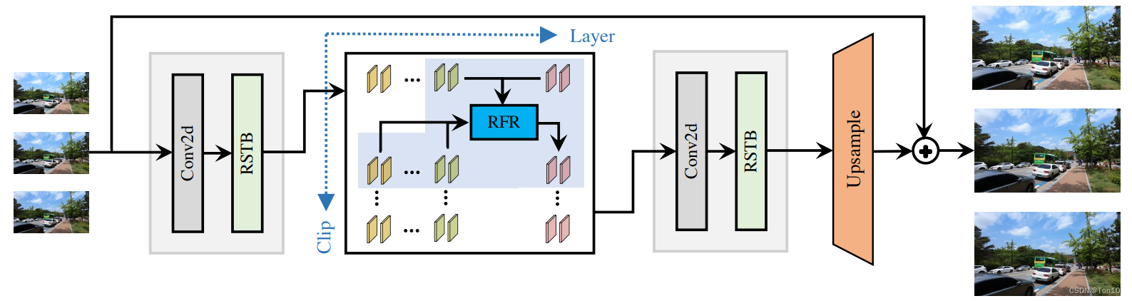
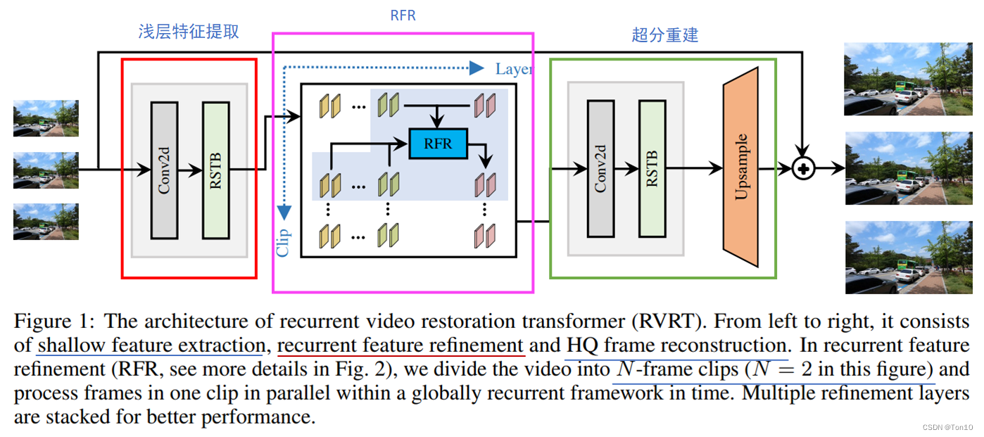
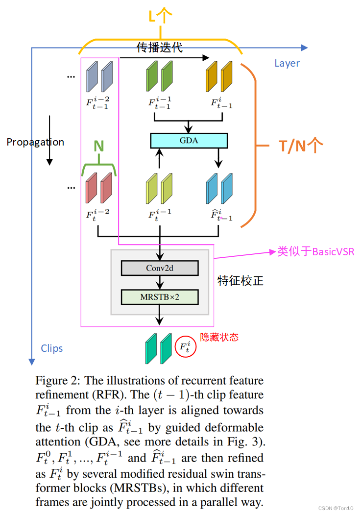
 本文介绍了一种名为RVRT的新型视频超分辨率(VSR)模型,它结合了循环网络和Transformer的优点。RVRT通过将序列划分为clips,并在每个clips内部使用Transformer进行并行处理,同时使用Guided Deformable Attention (GDA)进行视频对齐,以解决长距离特征捕获和计算效率的问题。实验表明,RVRT在视频超分辨率任务上实现了最优的性能与计算资源之间的平衡。
 最低0.47元/天 解锁文章


 721
721


 被折叠的 条评论
为什么被折叠?
被折叠的 条评论
为什么被折叠?
 到【灌水乐园】发言


