Tensorflow——TensorFlow基础

TensorFlow 基础

资料来源——TensorFlow官网¹
文章并不完整

Tensorflow是一个端到端的机器学习平台，它支持以下内容：

• 基于多维数组的数值计算（和NumPy类似）
• GPU和分布式处理
• 自动微分
• 模型构建，训练和输出
• 等等

张量（其实就是向量）

Tensorflow运行多维数组或张量表示对象tf.Tensor，其中最重要的参数分别是shap和dtype：

• Tensor.shap：表示张量沿每个轴的大小
• Tensor.dtype：表示张量中所有元素的数据类型

Tensorflow在张量上实行标准的数学运算，以及许多专门用于机器学习的运算
如果想要提高程序速度可以在GPU上运行，在CPU上进行大规模运算时速度比较慢

变量

tf.Tensor对象一般是不变的。可以使用tf.Variable存储模型权重（或是其他可变的状态）

自动微分

梯度下降和相关算法是当机器学习的基础。Tensorflow实现了自动微分，使用微积分来计算梯度。通常，你可以使用这个来计算模型的误差或损失相对于它权重的梯度
Tensorflow可以同时计算任意数量的非标量张量的梯度

图像和函数（tf.function)

你可以像使用Python库一样交互式地使用Tensorflow
Tensorflow也为性能优化、输出提供了工具

• 性能优化：加速训练和推导
• 输出：训练完之后可以保存自己的模型

你可以使用tf.function将纯TensorFlow代码与Python分离

@tf.function
def my_func(x):
	print('Tracing.\n')
	return tf.reduce_sum(x)

首先运行tf.function，尽管在Python中执行，它捕获了一个完整的优化图，表示函数中完成的TensorFlow计算。在后续调用中，TensorFlow只执行优化图，跳过任何非TensorFlow步骤。对于具有不同特征码（形状和数据类型）的输入，图形可能无法重复使用，因此会生成一个新的图形代替。

这些被捕获的图像提供了两个好处：

1. 大部分时候，它们能显著加快执行速度
2. 你可以使用tf.saved_model导出这些图像，然后在其他系统上运行，不需要安装Python

模块，层和模型

tf.Modules是一个管理tf.Variabel对象的类，并且tf.function对象在其上运行
tf.Modules类是支持两个重要功能所必须的：

1. 你可以使用tf.train.Checkpoint保存和恢复变量的值。
2. 你可以使用tf.saved_model导入和导出tf.Variable值和tf.function图像

下面有一个导出简单tf.Module对象的例子：

class MyModule(tf.Module):
	def __init__(self,value):
		self.weight = tf.Variable(value)
	
	@tf.function
	def multiply(self, x):
		return x * self.weight

mod = MyModule(3)
mod.multiply(tf.constant([1,2,3]))

保存模型：

save_path = './saved'
tf.saved_model.save(mod, save_path)

最后保存的模型独立于我们创建的代码

训练循环

现在，把这些一起建立一个基础模型并从头开始训练

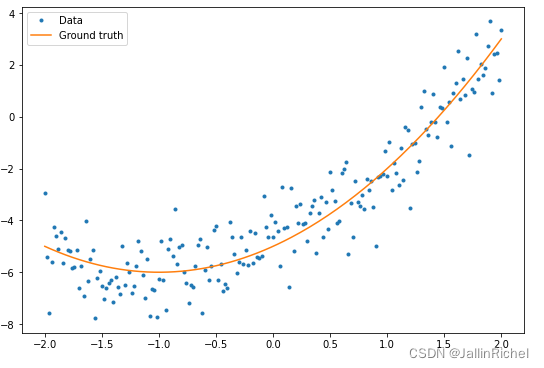
首先，创建一些样本数据，这会生成一个松散地沿着二次曲线的点云

import matplotlib
from matplotlib import pyplot as plt

matplotlib.rcParams['figure.figsize'] = [9,6]

x = tf.linspace(-2, 2, 201)
x = tf.cast(x, tf.float32)

def f(x):
  y = x**2 + 2*x - 5
  return y

y = f(x) + tf.random.normal(shape=[201])

plt.plot(x.numpy(), y.numpy(), '.', label='Data')
plt.plot(x, f(x),  label='Ground truth')
plt.legend();

建立模型：

class Model(tf.keras.Model):
  def __init__(self, units):
    super().__init__()
    self.dense1 = tf.keras.layers.Dense(units=units,
                                        activation=tf.nn.relu,
                                        kernel_initializer=tf.random.normal,
                                        bias_initializer=tf.random.normal)
    self.dense2 = tf.keras.layers.Dense(1)

  def call(self, x, training=True):
    # For Keras layers/models, implement `call` instead of `__call__`.
    x = x[:, tf.newaxis]
    x = self.dense1(x)
    x = self.dense2(x)
    return tf.squeeze(x, axis=1)
    
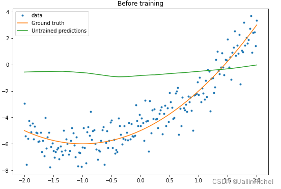
model = Model(64)

plt.plot(x.numpy(), y.numpy(), '.', label='data')
plt.plot(x, f(x),  label='Ground truth')
plt.plot(x, model(x), label='Untrained predictions')
plt.title('Before training')
plt.legend();

写一个基础训练循环：

variables = model.variables

optimizer = tf.optimizers.SGD(learning_rate=0.01)

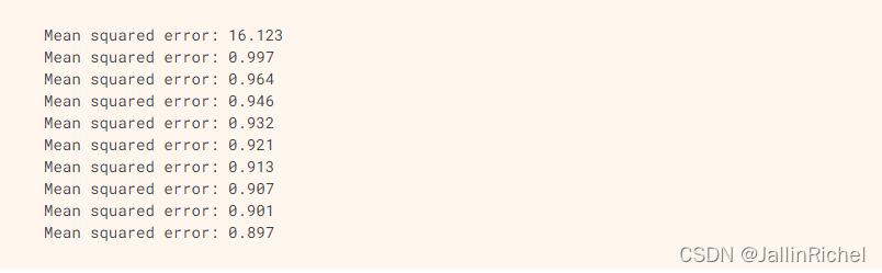
for step in range(1000):
  with tf.GradientTape() as tape:
    prediction = model(x)
    error = (y-prediction)**2
    mean_error = tf.reduce_mean(error)
  gradient = tape.gradient(mean_error, variables)
  optimizer.apply_gradients(zip(gradient, variables))

  if step % 100 == 0:
    print(f'Mean squared error: {mean_error.numpy():0.3f}')

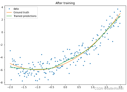
plt.plot(x.numpy(),y.numpy(), '.', label="data")
plt.plot(x, f(x),  label='Ground truth')
plt.plot(x, model(x), label='Trained predictions')
plt.title('After training')
plt.legend();

这是可行的，但是在tf.keras模块中提供了通用训练程序，所以在自己写训练循环之前不妨先考虑已经提供的。用Model.compile和Model.fit方法实施你的训练循环

new_model = Model(64)

new_model.compile(
    loss=tf.keras.losses.MSE,
    optimizer=tf.optimizers.SGD(learning_rate=0.01))

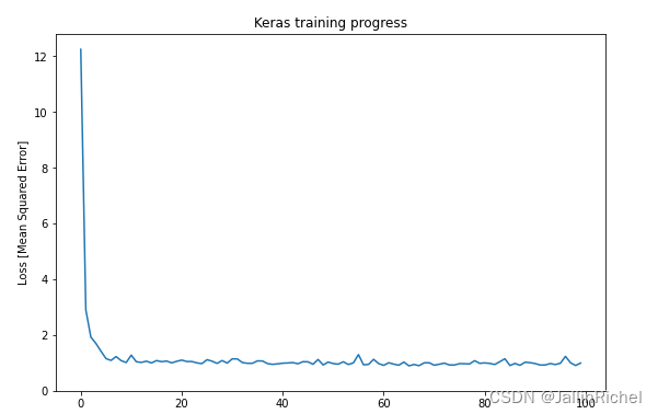
history = new_model.fit(x, y,
                        epochs=100,
                        batch_size=32,
                        verbose=0)

model.save('./my_model')

plt.plot(history.history['loss'])
plt.xlabel('Epoch')
plt.ylim([0, max(plt.ylim())])
plt.ylabel('Loss [Mean Squared Error]')
plt.title('Keras training progress');

---

1. 官方教程 ↩︎