matlab图像处理 Introduction to MATLAB

Introduction to MATLAB

The MATLAB environment and programming language will be used intensively during the MPV labs. In case you are not familiar with basics of this environment, study the following parts of the "Getting started with MATLAB (MathWorks)":

• Matrices and Arrays - (Expressions, Working with Matrices, More About Matrices and Arrays)
• Graphics - (Editing Plots, Mesh and Surface Plots, Images)
• Programming - (Flow Control, Other Data Structures, Scripts and Functions)

(home study)

Another useful tutorials are:

"Getting started with MATLAB (Indiana University)"

"Matlab Tutorial (Clarkson University)"

Revision of Basics of Image Processing

Another important precondition of the MPV labs is the basics of image processing in MATLAB.

Convolution, Image Smoothing and Gradient

• The Gaussian function is often used in image processing as a model of ideal point, low pass filter for noise reduction or so-called windowing function for weighting contribution of points in the neighbourhood. Write an implementation of the function  G=gauss(x,sigma) that computes discrete samples of Gaussian
  
  in points given by vector with variance   and zero mean.
• Implement function  D=dgauss(x,sigma) that returns a discrete samples of first derivation of Gaussian
  
  v in points given by vector with variance   and zero mean.
• Get acquainted with the function  conv2.
• The effect of filtering with Gaussian can be studied on an impulse response:

  sigma = 6.0;
  x = [-ceil(3.0*sigma):ceil(3.0*sigma)];
  G = gauss(x, sigma);
  D = dgauss(x, sigma);
  imp = zeros(51); imp(25,25) = 255;
  out = conv2(G,G,imp);
  ...
  
  imagesc(out); % or surf(out);

  try to find out impulse responses of other combinations of the Gaussian and its derivatives.

• Examples of impulse responses: 
   
  
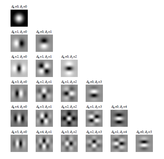
• Write a function  out=gaussfilter(in,sigma) that implements smoothing of an input image  in with a Gaussian filter of width  2*(sigma*3.0)+1 and variance   and returns the smoothed image  out (e.g.  Lenna). Exploit the separability property of Gaussian filter and implement the smoothing as two convolutions with one dimensional Gaussian filter (see function  conv2).
• Modify function gaussfilter to a new function  [dx,dy]=gaussderiv(in,sigma) that returns the estimate of the gradient (gx, gy) in each point of the input image  in (MxN matrix) after smoothing with Gaussian with variance  . Use either first derivative of Gaussian or the convolution and symmetric difference to estimate the gradient.
• Implement function  [dxx,dxy,dyy]=gaussderiv2(in,sigma) that returns all second derivatives of input image  in (MxN matrix) after smoothing with Gaussian of variance  .

References

Additional study material: chapters [3,4,5] on the Gaussian function, its derivatives and their role in image processing

Geometric Transformations and Interpolation of the Image

• Implement function  A=affine(x1,y1,x2,y2,x3,y3) that returns 3×3 transformation matrix A which transforms point in homogeneous coordinates from canonical coordinate system into image: (0,0,1)→(x1,y1,1), (1,0,1)→(x2,y2,1), (0,1,1)→(x3,y3,1). 
  
  
• Write function  out=affinetr(in,A,ps,ext) that warps a patch from image  in (MxN matrix) into canonical coordinate system. Affine transformation matrix  A (3×3 elements) is a transformation matrix from the canonical coordinate system into image from previous task. The parameter  ps defines the dimensions of the output image (the length of each side) and  ext is a real number that defines the extent of the patch in coordinates of the canonical coordinate system. E.g. out=affinetr(in,A,41,3.0), returns the patch of size 41×41 pixels that corresponds to the rectangle (-3.0,-3.0)x(3.0,3.0) in the canonical coordinate system. Top left corner of the image has coordinates (0,0). Use bilinear interpolation for image warping. Check the functionality on  image. 
  
  

What should you upload?

All the functions implemented in tasks of this lab in Matlab: gauss.m, dgauss.m, gaussfilter.m, gaussderiv.m, gaussderiv2.m,affine.m a affinetr.m upload into the upload system as a .zip archive. Keep all functions in the root of the .zip archive together with all helper your functions required. Follow closely the specification and order of the input/output arguments.

References

Geometric transformations - hierarchy of transformations, homogeneous coordinates
Geometric transformations - review of course Digital image processing

Checking Your Results

You can check results of the functions required in this lab using the Matlab function publish. Copy the test script test.minto MATLAB path (directory with implemented functions) a run. Compare your results to the reference solution (updated 16.2.2011, 18:10).

from: https://cw.fel.cvut.cz/wiki/courses/ae4m33mpv/labs/1_intro/start