二手车价格预测task03:特征工程_二手车特征 1+2-优快云博客

该博客介绍了二手车价格预测中的特征工程实践，包括数据导入、异常值处理、特征构造如时间特征、邮编特征、销量统计量和数据分桶，以及对power和kilometer特征的分析和归一化。此外，还涉及特征筛选方法如过滤式、包裹式，并强调了特征工程在提升模型性能中的关键作用。

摘要生成于 C知道，由 DeepSeek-R1 满血版支持，前往体验 >

二手车价格预测task03:特征工程

1.学习了operator模块operator.itemgetter()函数
2.学习了箱线图
3.了解了特征工程的方法 (内容介绍)
4.敲代码学习,加注解

以下是代码

代码示例

1.导入数据

import pandas as pd
import numpy as np
import matplotlib.pyplot as plt
import seaborn as sns
import warnings
warnings.filterwarnings('ignore')
%matplotlib inline
# 这个之前没见过
from operator import itemgetter

train = pd.read_csv('car_train_0110.csv', sep=' ')
test = pd.read_csv('car_testA_0110.csv',sep= ' ')

train.shape, test.shape

((250000, 40), (50000, 39))

train.columns # 看下列名

Index(['SaleID', 'name', 'regDate', 'model', 'brand', 'bodyType', 'fuelType',
       'gearbox', 'power', 'kilometer', 'notRepairedDamage', 'regionCode',
       'seller', 'offerType', 'creatDate', 'price', 'v_0', 'v_1', 'v_2', 'v_3',
       'v_4', 'v_5', 'v_6', 'v_7', 'v_8', 'v_9', 'v_10', 'v_11', 'v_12',
       'v_13', 'v_14', 'v_15', 'v_16', 'v_17', 'v_18', 'v_19', 'v_20', 'v_21',
       'v_22', 'v_23'],
      dtype='object')

2.异常值处理 (删除或者用最大值填充)

# 一个异常值处理的代码,可以随便调用
def outliers_proc(data,col_name,scale=3):
    """
    用于清洗异常值，默认用 box_plot（scale=3）进行清洗
    :param data: 接收 pandas 数据格式
    :param col_name: pandas 列名
    :param scale: 尺度
    :return:
    """
    def box_plot_outliers(data_ser, box_scale):
        """
        利用箱线图去除异常值
        :param data_ser: 接收 pandas.Series 数据格式
        :param box_scale: 箱线图尺度，
        :return:
        """
        iqr = box_scale * (data_ser.quantile(0.75) - data_ser.quantile(0.25)) # 像是一个阈值的定义
        val_low = data_ser.quantile(0.25) - iqr # 一列中的最小值
        val_up = data_ser.quantile(0.75) + iqr  # 一列中的最大值
        rule_low = (data_ser < val_low) # 小于最小值的设置为了0
        rule_up = (data_ser > val_up)   # 大于最小值的设置为了1
        return (rule_low, rule_up), (val_low, val_up)
    
    # 这里是删除异常值 -- 不建议删除吧..
    data_n = data.copy()
    data_series = data_n[col_name] # 得到了这一列数据
    rule, value = box_plot_outliers(data_series, box_scale=scale)
    index = np.arange(data_series.shape[0])[rule[0] | rule[1]]
    print("Delete number is: {}".format(len(index)))
    data_n = data_n.drop(index)
    data_n.reset_index(drop=True, inplace=True)
    print("Now column number is: {}".format(data_n.shape[0]))
    index_low = np.arange(data_series.shape[0])[rule[0]]
    outliers = data_series.iloc[index_low]
    print("Description of data less than the lower bound is:")
    print(pd.Series(outliers).describe())
    index_up = np.arange(data_series.shape[0])[rule[1]]
    outliers = data_series.iloc[index_up]
    print("Description of data larger than the upper bound is:")
    print(pd.Series(outliers).describe())
    
    
#     # 这里是异常值的填充 -- 实现这个替换上面直接删除的那个
#     data_n = data.copy()
#     data_series = data_n[col_name] # 得到了这一列数据
#     rule, value = box_plot_outliers(data_series, box_scale=scale)
#     index = np.arange(data_series.shape[0])[rule[0] | rule[1]]
#     print("Delete number is: {}".format(len(index)))
#     data_n = data_n.drop(index)
#     data_n.reset_index(drop=True, inplace=True)
#     print("Now column number is: {}".format(data_n.shape[0]))
#     index_low = np.arange(data_series.shape[0])[rule[0]]
#     outliers = data_series.iloc[index_low]
#     print("Description of data less than the lower bound is:")
#     print(pd.Series(outliers).describe())
#     index_up = np.arange(data_series.shape[0])[rule[1]]
#     outliers = data_series.iloc[index_up]
#     print("Description of data larger than the upper bound is:")
#     print(pd.Series(outliers).describe())
    
    
    
    fig, ax = plt.subplots(1, 2, figsize=(10, 7))
    sns.boxplot(y=data[col_name], data=data, palette="Set1", ax=ax[0])
    sns.boxplot(y=data_n[col_name], data=data_n, palette="Set1", ax=ax[1])
    return data_n

# 可以删掉一些异常数据，以 power 为例。  
# 这里删不删可以自行判断
# 但是要注意 test 的数据不能删 

train = outliers_proc(train, 'power', scale=3)

Delete number is: 1290
Now column number is: 248710
Description of data less than the lower bound is:
count    0.0
mean     NaN
std      NaN
min      NaN
25%      NaN
50%      NaN
75%      NaN
max      NaN
Name: power, dtype: float64
Description of data larger than the upper bound is:
count     1290.000000
mean      1104.958915
std       2373.619469
min        392.000000
25%        420.000000
50%        476.000000
75%        579.000000
max      20000.000000
Name: power, dtype: float64

在这里插入图片描述

# 删除所有数值型特征中的异常数据 -->这里最好不要删除,可以尝试用最大值和最小值替换异常值
numeric_features = ['power', 'kilometer', 'v_0', 'v_1', 'v_2', 'v_3', 'v_4', 'v_5', 'v_6', 'v_7', 'v_8', 'v_9', 'v_10', 'v_11', 'v_12', 'v_13','v_14' ]

# 这样会有太多图, 会删除太多数据,也不合适
# for fea in numeric_features:
#     train = outliers_proc(train, fea, scale=3)

3.特征构造

# 训练集和测试集放在一起，方便构造特征
train['train']=1
test['train']=0

train.head()

	SaleID	name	regDate	model	brand	bodyType	fuelType	gearbox	power	kilometer	...	v_15	v_16	v_17	v_18	v_19	v_20	v_21	v_22	v_23	train
0	134890	734	20160002	13.0	9	NaN	0.0	1.0	0	15.0	...	0.000000	18.763832	-1.512063	-1.008718	-12.100623	-0.947052	9.077297	0.581214	3.945923	1
1	306648	196973	20080307	72.0	9	7.0	5.0	1.0	173	15.0	...	0.122335	-5.685612	-0.489963	-2.223693	-0.226865	-0.658246	-3.949621	4.593618	-1.145653	1
2	340675	25347	20020312	18.0	12	3.0	0.0	1.0	50	12.5	...	0.003345	-3.295700	1.816499	3.554439	-0.683675	0.971495	2.625318	-0.851922	-1.246135	1
3	57332	5382	20000611	38.0	8	7.0	0.0	1.0	54	15.0	...	0.000000	-3.405521	1.497826	4.782636	0.039101	1.227646	3.040629	-0.801854	-1.251894	1
4	265235	173174	20030109	87.0	0	5.0	5.0	1.0	131	3.0	...	0.001655	-4.475429	0.124138	1.364567	-0.319848	-1.131568	-3.303424	-1.998466	-1.279368	1

5 rows × 41 columns

test.head()

	SaleID	name	regDate	model	brand	bodyType	fuelType	gearbox	power	kilometer	...	v_15	v_16	v_17	v_18	v_19	v_20	v_21	v_22	v_23
0	720326	505	20060505	19.0	13	7.0	0.0	1.0	90	8.0	...	0.105382	-5.998993	0.147048	-1.902847	0.348990	2.324961	3.343910	4.048742	-1.431822
1	714316	1836	20010301	5.0	5	3.0	4.0	1.0	75	15.0	...	0.000000	-3.287221	2.081317	2.937052	-0.123018	1.202395	3.570743	-1.180587	-1.348598
2	704693	212291	20170610	6.0	18	NaN	5.0	0.0	150	15.0	...	0.000000	4.368218	8.252188	-4.136109	-13.334970	-4.444620	-0.706978	-1.720218	3.569112
3	624972	1345	19820005	215.0	32	7.0	0.0	1.0	0	6.0	...	0.100883	-2.537486	0.513955	4.414962	0.357685	2.700732	5.323602	6.085956	-0.900585
4	669753	1428	20060205	30.0	4	7.0	5.0	1.0	122	15.0	...	0.002509	-6.197633	-0.191814	-1.224360	-0.326985	2.254931	4.183037	-2.574004	0.014203

5 rows × 40 columns

# 将训练集和测试集的数据拼接到一起 : pd.concat()函数
data = pd.concat([train, test], ignore_index=True, sort=False)

data.head().append(data.tail())

	SaleID	name	regDate	model	brand	bodyType	fuelType	gearbox	power	kilometer	...	v_15	v_16	v_17	v_18	v_19	v_20	v_21	v_22	v_23	train
0	134890	734	20160002	13.0	9	NaN	0.0	1.0	0	15.0	...	0.000000	18.763832	-1.512063	-1.008718	-12.100623	-0.947052	9.077297	0.581214	3.945923	1
1	306648	196973	20080307	72.0	9	7.0	5.0	1.0	173	15.0	...	0.122335	-5.685612	-0.489963	-2.223693	-0.226865	-0.658246	-3.949621	4.593618	-1.145653	1
2	340675	25347	20020312	18.0	12	3.0	0.0	1.0	50	12.5	...	0.003345	-3.295700	1.816499	3.554439	-0.683675	0.971495	2.625318	-0.851922	-1.246135	1
3	57332	5382	20000611	38.0	8	7.0	0.0	1.0	54	15.0	...	0.000000	-3.405521	1.497826	4.782636	0.039101	1.227646	3.040629	-0.801854	-1.251894	1
4	265235	173174	20030109	87.0	0	5.0	5.0	1.0	131	3.0	...	0.001655	-4.475429	0.124138	1.364567	-0.319848	-1.131568	-3.303424	-1.998466	-1.279368	1
298705	375033	3803	20010407	6.0	29	5.0	0.0	0.0	186	10.0	...	0.000372	-3.397636	0.940183	4.115667	0.146320	-2.348749	-2.636560	-0.965214	-1.097192	0
298706	406556	28500	20071001	130.0	10	2.0	0.0	0.0	272	7.0	...	0.116459	-7.055336	-1.260228	-4.937979	0.881517	-1.590285	-3.495608	3.301887	3.947193	0
298707	511668	98383	19980102	23.0	10	4.0	0.0	1.0	190	0.5	...	0.067015	-4.916501	0.507919	-0.035475	0.256285	0.734084	0.779931	1.822416	5.012697	0
298708	533139	1489	20031001	70.0	1	7.0	4.0	NaN	101	15.0	...	0.000000	-0.424439	3.893203	-0.146884	1.830694	18.008141	-2.513048	-3.310876	-1.589404	0
298709	592803	994	20070407	76.0	0	4.0	5.0	NaN	0	15.0	...	0.110924	-1.422750	2.749703	-2.160718	0.838089	17.664283	-5.802325	3.063008	-1.308131	0

10 rows × 41 columns

1.时间特征构造

# 使用时间：data['creatDate'] - data['regDate']，反应汽车使用时间，一般来说价格与使用时间成反比
# 不过要注意，数据里有时间出错的格式，所以我们需要 errors='coerce'
data['used_time'] = (pd.to_datetime(data['creatDate'], format='%Y%m%d', errors='coerce') - 
                            pd.to_datetime(data['regDate'], format='%Y%m%d', errors='coerce')).dt.days

# 看一下空数据，有 7721 个样本的时间是有问题的，我们可以选择删除，也可以选择放着。
# 但是这里不建议删除，因为删除缺失数据占总样本量过大 ?.
# 我们可以先放着，因为如果我们 XGBoost 之类的决策树，其本身就能处理缺失值，所以可以不用管；
data['used_time'].isnull().sum()

2.邮编特征构造 – 一般应该不知道这个特征信息

# 从邮编中提取城市信息，因为是德国的数据，所以参考德国的邮编，相当于加入了先验知识
# data['city'] = data['regionCode'].apply(lambda x : str(x)[:-3])

3.计算某品牌的销量统计量 – 害了一计算其他特征的统计量

# 这里要以 train 的数据计算统计量
train_gb = train.groupby("brand")
all_info = {}
for kind, kind_data in train_gb:
    info = {}
    kind_data = kind_data[kind_data['price'] > 0]
    info['brand_amount'] = len(kind_data)
    info['brand_price_max'] = kind_data.price.max()
    info['brand_price_median'] = kind_data.price.median()
    info['brand_price_min'] = kind_data.price.min()
    info['brand_price_sum'] = kind_data.price.sum()
    info['brand_price_std'] = kind_data.price.std()
    info['brand_price_average'] = round(kind_data.price.sum() / (len(kind_data) + 1), 2)
    all_info[kind] = info
brand_fe = pd.DataFrame(all_info).T.reset_index().rename(columns={"index": "brand"})
# data = data.merge(brand_fe, how='left', on='brand')
# 这里用上面那种方式会重复多出好多列
data = pd.merge(data,brand_fe,how='left', on='brand')

data.columns

Index(['SaleID', 'name', 'regDate', 'model', 'brand', 'bodyType', 'fuelType',
       'gearbox', 'power', 'kilometer', 'notRepairedDamage', 'regionCode',
       'seller', 'offerType', 'creatDate', 'price', 'v_0', 'v_1', 'v_2', 'v_3',
       'v_4', 'v_5', 'v_6', 'v_7', 'v_8', 'v_9', 'v_10', 'v_11', 'v_12',
       'v_13', 'v_14', 'v_15', 'v_16', 'v_17', 'v_18', 'v_19', 'v_20', 'v_21',
       'v_22', 'v_23', 'train', 'used_time', 'brand_amount', 'brand_price_max',
       'brand_price_median', 'brand_price_min', 'brand_price_sum',
       'brand_price_std', 'brand_price_average'],
      dtype='object')

4. 数据分桶

为什么要做数据分桶呢，原因有很多，= =
1. 离散后稀疏向量内积乘法运算速度更快，计算结果也方便存储，容易扩展；
1. 离散后的特征对异常值更具鲁棒性，如 age>30 为 1 否则为 0，对于年龄为 200 的也不会对模型造成很大的干扰；
1. LR 属于广义线性模型，表达能力有限，经过离散化后，每个变量有单独的权重，这相当于引入了非线性，能够提升模型的表达能力，加大拟合；
1. 离散后特征可以进行特征交叉，提升表达能力，由 M+N 个变量编程 M*N 个变量，进一步引入非线形，提升了表达能力；
1. 特征离散后模型更稳定，如用户年龄区间，不会因为用户年龄长了一岁就变化
当然还有很多原因，LightGBM 在改进 XGBoost 时就增加了数据分桶，增强了模型的泛化性

# 数据分桶 以 power 为例  -- 分成了30个桶
# 这时候我们的缺失值也进桶了，
bin = [i*10 for i in range(31)]
data['power_bin'] = pd.cut(data['power'], bin, labels=False)
data[['power_bin', 'power']].head()

	power_bin	power
0	NaN	0
1	17.0	173
2	4.0	50
3	5.0	54
4	13.0	131

data['power_bin'].nunique()

5.利用好了，就可以删掉原始数据了

data = data.drop(['creatDate', 'regDate',], axis=1)

print(data.shape)
data.columns

(298710, 48)





Index(['SaleID', 'name', 'model', 'brand', 'bodyType', 'fuelType', 'gearbox',
       'power', 'kilometer', 'notRepairedDamage', 'regionCode', 'seller',
       'offerType', 'price', 'v_0', 'v_1', 'v_2', 'v_3', 'v_4', 'v_5', 'v_6',
       'v_7', 'v_8', 'v_9', 'v_10', 'v_11', 'v_12', 'v_13', 'v_14', 'v_15',
       'v_16', 'v_17', 'v_18', 'v_19', 'v_20', 'v_21', 'v_22', 'v_23', 'train',
       'used_time', 'brand_amount', 'brand_price_max', 'brand_price_median',
       'brand_price_min', 'brand_price_sum', 'brand_price_std',
       'brand_price_average', 'power_bin'],
      dtype='object')

# 目前的数据其实已经可以给树模型使用了，所以我们导出一下
data.to_csv('task03_data_for_tree.csv', index=0) # index=0表示不要前面的索引列

# 读取出来看看数据
data_tree = pd.read_csv('task03_data_for_tree.csv')

data_tree

	SaleID	name	model	brand	bodyType	fuelType	gearbox	power	kilometer	notRepairedDamage	...	train	used_time	brand_amount	brand_price_max	brand_price_median	brand_price_min	brand_price_sum	brand_price_std	brand_price_average	power_bin
0	134890	734	13.0	9	NaN	0.0	1.0	0	15.0	NaN	...	1	NaN	11813.0	72500.0	1350.0	1.0	28249065.0	3067.406603	2391.15	NaN
1	306648	196973	72.0	9	7.0	5.0	1.0	173	15.0	1.0	...	1	2926.0	11813.0	72500.0	1350.0	1.0	28249065.0	3067.406603	2391.15	17.0
2	340675	25347	18.0	12	3.0	0.0	1.0	50	12.5	1.0	...	1	5125.0	4565.0	35500.0	2690.0	1.0	20232646.0	4804.870237	4431.15	4.0
3	57332	5382	38.0	8	7.0	0.0	1.0	54	15.0	1.0	...	1	5771.0	3273.0	99999.0	2100.0	1.0	15145456.0	5746.032111	4625.98	5.0
4	265235	173174	87.0	0	5.0	5.0	1.0	131	3.0	1.0	...	1	4806.0	51843.0	100000.0	2999.0	1.0	275586832.0	6226.472359	5315.69	13.0
...	...	...	...	...	...	...	...	...	...	...	...	...	...	...	...	...	...	...	...	...	...
298705	375033	3803	6.0	29	5.0	0.0	0.0	186	10.0	1.0	...	0	5470.0	1197.0	90500.0	4490.0	1.0	7887207.0	6407.870205	6583.65	18.0
298706	406556	28500	130.0	10	2.0	0.0	0.0	272	7.0	1.0	...	0	3095.0	23028.0	99999.0	4999.0	1.0	182980565.0	8429.058935	7945.66	27.0
298707	511668	98383	23.0	10	4.0	0.0	1.0	190	0.5	1.0	...	0	6648.0	23028.0	99999.0	4999.0	1.0	182980565.0	8429.058935	7945.66	18.0
298708	533139	1489	70.0	1	7.0	4.0	NaN	101	15.0	1.0	...	0	4567.0	21339.0	84911.0	5900.0	1.0	186533771.0	8877.868472	8741.04	10.0
298709	592803	994	76.0	0	4.0	5.0	NaN	0	15.0	1.0	...	0	3261.0	51843.0	100000.0	2999.0	1.0	275586832.0	6226.472359	5315.69	NaN

298710 rows × 48 columns

6.再构造一份特征供 LR NN之类的模型使用

之所以分开构造是因为，不同模型对数据集的要求不同

data # 删除异常值后数据少了很多emm.

	SaleID	name	model	brand	bodyType	fuelType	gearbox	power	kilometer	notRepairedDamage	...	train	used_time	brand_amount	brand_price_max	brand_price_median	brand_price_min	brand_price_sum	brand_price_std	brand_price_average	power_bin
0	134890	734	13.0	9	NaN	0.0	1.0	0	15.0	NaN	...	1	NaN	11813.0	72500.0	1350.0	1.0	28249065.0	3067.406603	2391.15	NaN
1	306648	196973	72.0	9	7.0	5.0	1.0	173	15.0	1.0	...	1	2926.0	11813.0	72500.0	1350.0	1.0	28249065.0	3067.406603	2391.15	17.0
2	340675	25347	18.0	12	3.0	0.0	1.0	50	12.5	1.0	...	1	5125.0	4565.0	35500.0	2690.0	1.0	20232646.0	4804.870237	4431.15	4.0
3	57332	5382	38.0	8	7.0	0.0	1.0	54	15.0	1.0	...	1	5771.0	3273.0	99999.0	2100.0	1.0	15145456.0	5746.032111	4625.98	5.0
4	265235	173174	87.0	0	5.0	5.0	1.0	131	3.0	1.0	...	1	4806.0	51843.0	100000.0	2999.0	1.0	275586832.0	6226.472359	5315.69	13.0
...	...	...	...	...	...	...	...	...	...	...	...	...	...	...	...	...	...	...	...	...	...
298705	375033	3803	6.0	29	5.0	0.0	0.0	186	10.0	1.0	...	0	5470.0	1197.0	90500.0	4490.0	1.0	7887207.0	6407.870205	6583.65	18.0
298706	406556	28500	130.0	10	2.0	0.0	0.0	272	7.0	1.0	...	0	3095.0	23028.0	99999.0	4999.0	1.0	182980565.0	8429.058935	7945.66	27.0
298707	511668	98383	23.0	10	4.0	0.0	1.0	190	0.5	1.0	...	0	6648.0	23028.0	99999.0	4999.0	1.0	182980565.0	8429.058935	7945.66	18.0
298708	533139	1489	70.0	1	7.0	4.0	NaN	101	15.0	1.0	...	0	4567.0	21339.0	84911.0	5900.0	1.0	186533771.0	8877.868472	8741.04	10.0
298709	592803	994	76.0	0	4.0	5.0	NaN	0	15.0	1.0	...	0	3261.0	51843.0	100000.0	2999.0	1.0	275586832.0	6226.472359	5315.69	NaN

298710 rows × 48 columns

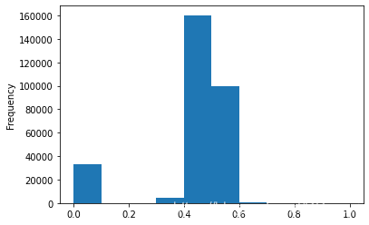
1.对power特征进行分析

data['power'].plot.hist()

<AxesSubplot:ylabel='Frequency'>

在这里插入图片描述

我们刚刚已经对 train 进行异常值处理了，但是现在还有这么奇怪的分布是因为 test 中的 power 异常值，
所以我们其实刚刚 train 中的 power 异常值不删为好，可以用长尾分布截断来代替

train['power'].plot.hist()

<AxesSubplot:ylabel='Frequency'>

在这里插入图片描述

data.shape,train.shape,test.shape

((298710, 48), (248710, 41), (50000, 40))

test['power'].plot.hist()

<AxesSubplot:ylabel='Frequency'>

在这里插入图片描述

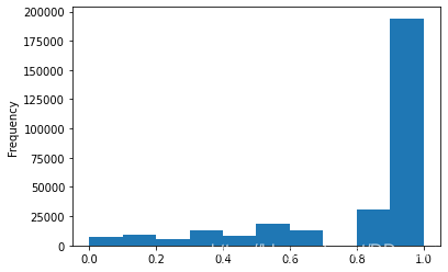
# 我们对其取 log，在做归一化
from sklearn import preprocessing

# min_max_scaler = preprocessing.MinMaxScaler() # 这个没用到
data['power'] = np.log(data['power'] + 1) 
data['power'] = ((data['power'] - np.min(data['power'])) / (np.max(data['power']) - np.min(data['power'])))

data['power'].plot.hist()

<AxesSubplot:ylabel='Frequency'>

在这里插入图片描述

2.对kilometer特征进行分析

# km 的比较正常，应该是已经做过分桶了
data['kilometer'].plot.hist()

<AxesSubplot:ylabel='Frequency'>

在这里插入图片描述

# 所以我们可以直接做归一化
data['kilometer'] = ((data['kilometer'] - np.min(data['kilometer'])) / 
                        (np.max(data['kilometer']) - np.min(data['kilometer'])))
data['kilometer'].plot.hist()

<AxesSubplot:ylabel='Frequency'>

在这里插入图片描述

3.对刚刚构造的特征进行归一化

# 除此之外 还有我们刚刚构造的统计量特征：
# 'brand_amount', 'brand_price_average', 'brand_price_max',
# 'brand_price_median', 'brand_price_min', 'brand_price_std',
# 'brand_price_sum'
# 这里不再一一举例分析了，直接做变换，
def max_min(x):
    return (x - np.min(x)) / (np.max(x) - np.min(x))

data['brand_amount'] = ((data['brand_amount'] - np.min(data['brand_amount'])) / 
                        (np.max(data['brand_amount']) - np.min(data['brand_amount'])))
data['brand_price_average'] = ((data['brand_price_average'] - np.min(data['brand_price_average'])) / 
                               (np.max(data['brand_price_average']) - np.min(data['brand_price_average'])))
data['brand_price_max'] = ((data['brand_price_max'] - np.min(data['brand_price_max'])) / 
                           (np.max(data['brand_price_max']) - np.min(data['brand_price_max'])))
data['brand_price_median'] = ((data['brand_price_median'] - np.min(data['brand_price_median'])) /
                              (np.max(data['brand_price_median']) - np.min(data['brand_price_median'])))
data['brand_price_min'] = ((data['brand_price_min'] - np.min(data['brand_price_min'])) / 
                           (np.max(data['brand_price_min']) - np.min(data['brand_price_min'])))
data['brand_price_std'] = ((data['brand_price_std'] - np.min(data['brand_price_std'])) / 
                           (np.max(data['brand_price_std']) - np.min(data['brand_price_std'])))
data['brand_price_sum'] = ((data['brand_price_sum'] - np.min(data['brand_price_sum'])) / 
                           (np.max(data['brand_price_sum']) - np.min(data['brand_price_sum'])))

4.对类别特征进行 OneEncoder

data = pd.get_dummies(data, columns=['model', 'brand', 'bodyType', 'fuelType',
                                     'gearbox', 'notRepairedDamage', 'power_bin'])

data.shape

(298710, 381)

data.columns

Index(['SaleID', 'name', 'power', 'kilometer', 'regionCode', 'seller',
       'offerType', 'price', 'v_0', 'v_1',
       ...
       'power_bin_20.0', 'power_bin_21.0', 'power_bin_22.0', 'power_bin_23.0',
       'power_bin_24.0', 'power_bin_25.0', 'power_bin_26.0', 'power_bin_27.0',
       'power_bin_28.0', 'power_bin_29.0'],
      dtype='object', length=381)

# 这份数据可以给 LR 用
data.to_csv('task03_data_for_lr.csv', index=0)

4.特征筛选

1.过滤式

# 相关性分析 -- spearman方法
print(data['power'].corr(data['price'], method='spearman'))
print(data['kilometer'].corr(data['price'], method='spearman'))
print(data['brand_amount'].corr(data['price'], method='spearman'))
print(data['brand_price_average'].corr(data['price'], method='spearman'))
print(data['brand_price_max'].corr(data['price'], method='spearman'))
print(data['brand_price_median'].corr(data['price'], method='spearman'))

# 当然也可以直接看图 -- 这里应该写出来price这个特征
data_numeric = data[['power', 'kilometer', 'brand_amount', 'brand_price_average', 
                     'brand_price_max', 'brand_price_median','price']]
correlation = data_numeric.corr()

f , ax = plt.subplots(figsize = (7, 7))
plt.title('Correlation of Numeric Features with Price',y=1,size=16)
sns.heatmap(correlation,square = True,  vmax=0.8)

在这里插入图片描述

上传csdn图片不显示即将jupyter转成md的方法

将jupyter转成.md的方法
jupyter nbconvert --to markdown “task03_特征工程.ipynb”
会得到一个md和一个含有很多图片的文件夹
上传至csdn时,无法显示图片,因为图片在本地
需要为图片整个图床
https://blog.youkuaiyun.com/qq_20493631/article/details/109425496 写完这个看看这个博客实现它

2.包裹式

# !pip install mlxtend

# k_feature 太大会很难跑，没服务器，所以提前 interrupt 了
from mlxtend.feature_selection import SequentialFeatureSelector as SFS
from sklearn.linear_model import LinearRegression
sfs = SFS(LinearRegression(),
           k_features=10,
           forward=True,
           floating=False,
           scoring = 'r2',
           cv = 0)
x = data.drop(['price'], axis=1)
x = x.fillna(0)
y = data['price']
sfs.fit(x, y)
sfs.k_feature_names_

# 画出来，可以看到边际效益
from mlxtend.plotting import plot_sequential_feature_selection as plot_sfs
import matplotlib.pyplot as plt
fig1 = plot_sfs(sfs.get_metric_dict(), kind='std_dev')
plt.grid()
plt.show()

3.嵌入式 – 暂无

经验总结

特征工程是比赛中最至关重要的的一块，特别的传统的比赛，大家的模型可能都差不多，调参带来的效果增幅是非常有限的，但特征工程的好坏往往会决定了最终的排名和成绩。

特征工程的主要目的还是在于将数据转换为能更好地表示潜在问题的特征，从而提高机器学习的性能。比如，异常值处理是为了去除噪声，填补缺失值可以加入先验知识等。

特征构造也属于特征工程的一部分，其目的是为了增强数据的表达。

有些比赛的特征是匿名特征，这导致我们并不清楚特征相互直接的关联性，这时我们就只有单纯基于特征进行处理，比如装箱，groupby，agg
等这样一些操作进行一些特征统计，此外还可以对特征进行进一步的 log，exp
等变换，或者对多个特征进行四则运算（如上面我们算出的使用时长），多项式组合等然后进行筛选。由于特性的匿名性其实限制了很多对于特征的处理，当然有些时候用
NN 去提取一些特征也会达到意想不到的良好效果。

对于知道特征含义（非匿名）的特征工程，特别是在工业类型比赛中，会基于信号处理，频域提取，丰度，偏度等构建更为有实际意义的特征，这就是结合背景的特征构建，在推荐系统中也是这样的，各种类型点击率统计，各时段统计，加用户属性的统计等等，这样一种特征构建往往要深入分析背后的业务逻辑或者说物理原理，从而才能更好的找到
magic。

当然特征工程其实是和模型结合在一起的，这就是为什么要为 LR NN
做分桶和特征归一化的原因，而对于特征的处理效果和特征重要性等往往要通过模型来验证。

总的来说，特征工程是一个入门简单，但想精通非常难的一件事。

特征工程目标

对于特征进行进一步分析，并对于数据进行处理
完成对于特征工程的分析，并对于数据进行一些图表或者文字总结并打卡

内容介绍

常见的特征工程包括：

异常处理：
通过箱线图（或 3-Sigma）分析删除异常值；
BOX-COX 转换（处理有偏分布）；
长尾截断；
特征归一化/标准化：

标准化（转换为标准正态分布）；
归一化（抓换到 [0,1] 区间）；
针对幂律分布，可以采用公式： $log(\frac{1+x}{1+median})$

数据分桶：
等频分桶；
等距分桶；
Best-KS 分桶（类似利用基尼指数进行二分类）；
卡方分桶；

缺失值处理：
不处理（针对类似 XGBoost 等树模型）；
删除（缺失数据太多）；
插值补全，包括均值/中位数/众数/建模预测/多重插补/压缩感知补全/矩阵补全等；
分箱，缺失值一个箱；

特征构造：
构造统计量特征，报告计数、求和、比例、标准差等；
时间特征，包括相对时间和绝对时间，节假日，双休日等；
地理信息，包括分箱，分布编码等方法；
非线性变换，包括 log/ 平方/ 根号等；
特征组合，特征交叉；
仁者见仁，智者见智。

特征筛选
过滤式（filter）：先对数据进行特征选择，然后在训练学习器，常见的方法有 Relief/方差选择发/相关系数法/卡方检验法/互信息法；
包裹式（wrapper）：直接把最终将要使用的学习器的性能作为特征子集的评价准则，常见方法有 LVM（Las Vegas Wrapper）；
嵌入式（embedding）：结合过滤式和包裹式，学习器训练过程中自动进行了特征选择，常见的有 lasso 回归；

降维
PCA/ LDA/ ICA；
特征选择也是一种降维。