


作者 | 微卷的大白 编辑 | 自动驾驶之心
原文链接:https://zhuanlan.zhihu.com/p/1952449084788029155
点击下方卡片,关注“自动驾驶之心”公众号

>>自动驾驶前沿信息获取→自动驾驶之心知识星球
本文只做学术分享,如有侵权,联系删文
前两天看到李飞飞 Worldlabs 新工作Mrable的时候,提到后面想多看一看 3DGS / 重建相关的工作。
但是知乎搜了一下发现,讲 3DGS 论文原理、改进的不少,我自己上半年也回顾过cuda kernel 源码:重温经典之 3DGS CUDA 源码解析 ,但是另一个常用的gsplat 开源库则基本无人 care。
官方 arxiv链接:https://arxiv.org/pdf/2409.06765
顺便一提,3DGS 虽然也有可训练的模型/高斯参数,但是和常规的深度学习模型、框架都有不小的差别。和 CV/自驾还算有点关系,毕竟也需要涉及坐标系转换、lidar 点云等,24年还有很多人在做自驾感知/端到端和 nerf/3dgs 的结合,但和 LLM / NLP 则是基本毫无关联,跟概率论我觉得关系也不大。如非必要,大模型er 慎重踩这个坑。
不过如果真的有小白要踩坑,gsplat 的文档和维护其实比gaussian-splatting 要稍微好一些,个人更推荐这个库。
相比3DGS 论文对应的 gaussian-splatting 库,nerfstudio-projectgsplat 是对官方库做了一些优化,可参考https://docs.gsplat.studio/main/migration/migration_inria.html 的说明。
(也还有OpenSplat 、gaustudio等不少框架,不过 opensplat 是基于 C++的,gsustudio 我不太了解)
搜 gsplat 的时候还意外发现这个:
就像最近的NeRF、Gsplat一样。
然后再过几年,如果发现生成质量一直上不去,或者算力要求巨高,凉了,那就没啥影响了。
如果效果做的特别好,各种控制技术越来越精巧,文字理解越来越到位,不仅没凉反而真的能取代光追渲染器了,有人就会宣称Diffusion Transformer是计算机图形学的奠基技术之一。然后大学图形学课上开始将Sora作为经典案例来讲,有学生实现简化版Sora作为小作业,企业招图形学工程师面试加入Diffusion Transformer相关的考题。作者:Raymond Fei
标题:OpenAI 的新视频生成模型 Sora 将对计算机图形学产生什么影响? 。
从从业者的角度,我是非常期待“世界模型”的应用能广泛一些,无论视频生成还是场景重建,现在发展都有点惨淡。吃肉是大佬的事儿,不过哪怕效果和应用场景能有 LLM 1/4,算法和Infra 的小卡拉米们也有机会喝点汤不是(手动狗头)。俺真不太想换赛道去卷 LLM....
gsplat 文档简读
Data Conventions
四元数计算平移旋转
第一次接触这玩意是大二做智能车的时候...在单片机解陀螺仪位姿...回忆杀说来就来
相机坐标系和世界坐标系转换

gsplat 还强调其支持超广角畸变和卷帘快门的相机模型(好吧又是一波智能车比赛的回忆杀,自己学的东西是真杂)
Compression
gsplat 提供的高斯球存储压缩功能,文档介绍可以将 1M 的高斯球参数从 236MB 压缩到 16.5MB,仅有 0.5dB 的 PSNR 损失,原理包括
量化(Quantization):降低数值精度
排序(Sorting):提高压缩效率
K-means聚类:专门压缩球谐系数
PNG编码:利用图像压缩技术
Rasterization
https://docs.gsplat.studio/main/apis/rasterization.html 包含了 utils 中的多个操作
fully_fused_projection(): 3D→2D投影
isect_tiles() :tile相交检测
isect_offset_encode() :编码偏移量
rasterize_to_pixels() :像素光栅化
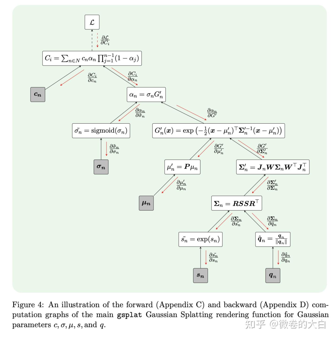
可以参考gsplat论文中的图来理解
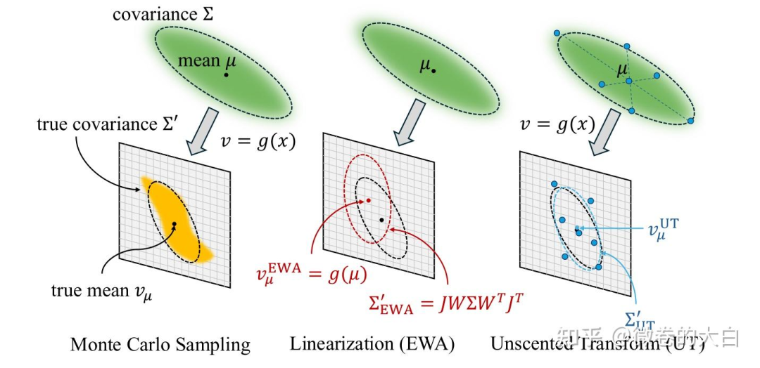
对于初识 3DGS 的同学,这个图对于理解协方差的投影也有些帮助:
文档列出来的几个公式涉及的知识点:
3D高斯参数:
:3D高斯的中心位置
:3D协方差矩阵(描述高斯的形状和方向)
:颜色属性
:不透明度
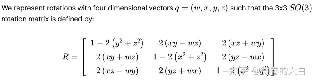
公式 是协方差矩阵的分解:
:缩放矩阵, 是缩放向量 ,控制高斯在三个轴上的大小
:旋转矩阵,由四元数 表示 ,控制高斯的方向
透视投影的雅可比矩阵 :

投影过程计算 2D 协方差:
计算 2D 投影的中心位置:
⎡fx  0  cx⎤   ⎡x_c/z_c⎤
μ' =  ⎢ 0  fy cy⎥ · ⎢y_c/z_c⎥
      ⎣ 0  0  1 ⎦   ⎣   1   ⎦
2D投影参数:
:投影后的2D中心位置
:投影后的2D协方差矩阵
:深度值
通过官方的 examples 可以对 rasterization的输入输出参数和shape 有一个基本概念
# define Gaussians
means = torch.randn((100, 3), device=device)
quats = torch.randn((100, 4), device=device)
scales = torch.rand((100, 3), device=device) * 0.1
colors = torch.rand((100, 3), device=device)
opacities = torch.rand((100,), device=device)

# define cameras
viewmats = torch.eye(4, device=device)[None, :, :]
Ks = torch.tensor([[300., 0., 150.], [0., 300., 100.], [0., 0., 1.]], device=device)[None, :, :]
width, height = 300, 200

# render
colors, alphas, meta = rasterization(means, quats, scales, opacities, colors, viewmats, Ks, width, height)

print (colors.shape, alphas.shape)
# torch.Size([1, 200, 300, 3]) torch.Size([1, 200, 300, 1])

print (meta.keys())
#dict_keys(['camera_ids', 'gaussian_ids', 'radii', 'means2d', 'depths', 'conics','opacities', 'tile_width', 'tile_height', 'tiles_per_gauss', 'isect_ids','flatten_ids', 'isect_offsets', 'width', 'height', 'tile_size'])
Densification
高斯球可以通过多种方式初始化,比如利用点云 SfM 初始化,但其并不像很多深度学习 Model 一样初始化后参数量就 Fix 下来了,在 3DGS 后续的训练中,高斯球的数量还会有变化,即 3DGS 论文中的 Adaptive Density Control,不同论文/方法会对应不同的更新策略,常规的比如分裂、复制、裁剪。
gsplat将高斯的密集化和修剪过程抽象为 策略(Strategy),从代码来看包括以下关键过程:
check_sanity():使用检查参数和优化器的格式是否正确initialize_state():初始化策略状态step_pre_backward():反向传播前的回调step_post_backward():反向传播后的回调
from gsplat import DefaultStrategy, rasterization

# Define Gaussian parameters and optimizers
params: Dict[str, torch.nn.Parameter] | torch.nn.ParameterDict = ...
optimizers: Dict[str, torch.optim.Optimizer] = ...

# Initialize the strategy
strategy = DefaultStrategy()

# Check the sanity of the parameters and optimizers
strategy.check_sanity(params, optimizers)

# Initialize the strategy state
strategy_state = strategy.initialize_state()

# Training loop
for step in range(1000):
    # Forward pass
    render_image, render_alpha, info = rasterization(...)

    # 策略前处理(收集统计信息)
    strategy.step_pre_backward(params, optimizers, strategy_state, step, info)

    # Compute the loss and Backward pass
    loss = ...
    loss.backward()

     # 策略后处理(执行实际的分裂/修剪)
    strategy.step_post_backward(params, optimizers, strategy_state, step, info)
DefaultStrategy 对应3DGS 论文的默认策略,包括:
复制高斯球:
触发条件: high image plane gradients and small scales.
原理:高梯度 说明该区域重建误差大,需要更多高斯;小尺度:说明是精细结构,不适合分裂(会破坏细节)。所以使用复制而非分裂:保留原有细节结构,在附近增加高斯球密度
分裂高斯球:
触发条件:high image plane gradients and large scales.
原理:大高斯难以精确表示复杂几何,所以通过分离,用多个小高斯更好地拟合局部细节。
修剪高斯球:
触发条件:low opacity.
原理: 低透明度的高斯球对图像贡献小,
重置高斯球到低透明度:
触发条件:定期触发(对应 reset_every 参数)
原理:防止部分高斯球不透明度过早收敛到 1,让不同高斯球重新展开竞争。
MCMCStrategy 对应另一种常用的方法https://arxiv.org/abs/2404.09591,gsplat 也给出了mcmc 的 demo : https://github.com/nerfstudio-project/gsplat/blob/main/examples/benchmarks/mcmc_4gpus.sh
Utils
https://docs.gsplat.studio/main/apis/utils.html
提供了更基础的 Python API 操作,以 rasterize_to_pixels 为例,可以直接from gsplat import rasterize_to_pixels
通过 gsplat/init.py 可以找到其函数定义在:https://github.com/nerfstudio-project/gsplat/blob/main/gsplat/cuda/_wrapper.py 中,类型检查之后,就是调用 cuda kernel 了,前向和反向对应两个 kernel:
fwd 在 https://github.com/nerfstudio-project/gsplat/blob/main/gsplat/cuda/csrc/RasterizeToPixels3DGSFwd.cu# L191
bwd 在 https://github.com/nerfstudio-project/gsplat/blob/main/gsplat/cuda/csrc/RasterizeToPixels3DGSBwd.cu
kernel 和原始的 gs 并无多大区别
参数转换
spherical_harmonics():计算球谐函数,将球谐系数转换为RGB颜色支持可选的mask来跳过部分计算
quat_scale_to_covar_preci():将四元数和缩放转换为协方差和精度矩阵可选择只计算其中一个(节省计算)
支持返回上三角形式(压缩存储)
projection 相关:
proj():将高斯球投影到2D像素空间(支持透视和正交投影)支持多种相机模型:
pinhole、ortho、fisheye、ftheta
fully_fused_projection()核心函数,融合了计算协方差、世界到相机空间变换、投影到2D多个操作。支持
packed模式(内存优化)支持
sparse_grad(稀疏梯度)自动过滤视锥体外的高斯
支持视角相关的不透明度补偿
world_to_cam():将高斯从世界坐标系转换到相机坐标系
tile 相关
isect_tiles():将投影到 2D 空间的高斯球映射到与其相交的像素 tile支持排序和分段排序
返回每个高斯相交的瓦片数和相交ID
isect_offset_encode():将相交ID编码为偏移量,用于后续的光栅化操作
光栅化渲染
rasterize_to_pixels():将高斯光栅化到像素支持背景色和遮罩
支持absgrad(绝对梯度计算)
rasterize_to_indices_in_range():迭代光栅化可以分批处理高斯(从近到远)
返回高斯-像素相交的索引
单卡训练
运行脚本:
CUDA_VISIBLE_DEVICES=5 python examples/simple_trainer.py default \
    --data_dir data/360_v2/garden/ --data_factor 4 \
    --result_dir ./results/garden \
    --packed
核心的 rasterize_to_pixels 调用栈如下,从外到内大概过一下

训练迭代循环
https://github.com/nerfstudio-project/gsplat/blob/main/examples/simple_trainer.py# L601
def train(self):
    for step in range(max_steps):
        # 1. 数据准备
        data = next(trainloader_iter)
        pixels = data["image"] / 255.0

        # 2. 可选的一些优化配置,还有 depth_loss, pose_noise等
        if cfg.pose_opt:
            camtoworlds = self.pose_adjust(camtoworlds, image_ids)

        # 3. 渲染
        renders, alphas, info = self.rasterize_splats(...)

        # 4. 策略前处理(收集统计)
        self.cfg.strategy.step_pre_backward(
            params=self.splats, state=self.strategy_state, info=info
        )

        # 5. 损失计算
        l1loss = F.l1_loss(colors, pixels)
        ssimloss = 1.0 - fused_ssim(colors, pixels)
        loss = l1loss * (1.0 - cfg.ssim_lambda) + ssimloss * cfg.ssim_lambda

        # 6. 反向传播
        loss.backward()

        # 7. 稀疏梯度处理(如果启用)
        if cfg.sparse_grad:
            gaussian_ids = info["gaussian_ids"]
            for k in self.splats.keys():
                grad = self.splats[k].grad
                self.splats[k].grad = torch.sparse_coo_tensor(
                    indices=gaussian_ids[None],
                    values=grad[gaussian_ids],
                    size=self.splats[k].size()
                )

        # 8. 优化器步进
        for optimizer in self.optimizers.values():
            optimizer.step()
            optimizer.zero_grad()

        # 9. 策略后处理(执行分裂/修剪)
        self.cfg.strategy.step_post_backward(
            params=self.splats, state=self.strategy_state, info=info
        )
前向渲染 Runner.rasterize_splats()
def rasterize_splats(self, ...):
    # 1. 提取参数
    means = self.splats["means"]
    quats = self.splats["quats"]
    scales = torch.exp(self.splats["scales"])  # log空间
    opacities = torch.sigmoid(self.splats["opacities"])

    # 2. 处理颜色
    if self.cfg.app_opt:
        # 外观模型:有些模型 对于不同视角和图像ID,有颜色变化的处理逻辑
        colors = self.app_module(
            features=self.splats["features"],    # 高斯特征
            embed_ids=image_ids,                 # 图像ID(外观嵌入)
            dirs=dirs,                           # 视角方向
            sh_degree=sh_degree,                 # SH阶数
        )
    else:
        # 标准SH系数
        colors = torch.cat([self.splats["sh0"], self.splats["shN"]], 1)  # [N, K, 3]

    # 3. 光栅化
    # 参数可以参考前面的文档说明
    render_colors, render_alphas, info = rasterization(
        # 高斯参数
        means=means, quats=quats, scales=scales, opacities=opacities, colors=colors,
        # means([138766, 3]), quats([138766, 4]), scales([138766, 3])
        # 相机参数
        viewmats=torch.linalg.inv(camtoworlds),  # 世界到相机变换 # [C, 4, 4]
        Ks=Ks,  # [C, 3, 3]
        width=width, height=height,

        # 优化选项
        packed=self.cfg.packed,              # 内存优化模式
        sparse_grad=self.cfg.sparse_grad,    # 稀疏梯度
        absgrad=...,                         # 绝对梯度(用于密集化)

        # 渲染选项
        rasterize_mode=rasterize_mode,       # 抗锯齿模式
        distributed=self.world_size > 1,      # 分布式渲染
        camera_model=camera_model,            # 相机模型

        # 高级选项
        with_ut=self.cfg.with_ut,            # Unscented Transform
        with_eval3d=self.cfg.with_eval3d,    # 3D评估模式

        **kwargs,  # 其他参数(如sh_degree, render_mode等)
    )

    # 如果有 mask, 将对应颜色置为 0
    if masks is not None:
         render_colors[~masks] = 0

    return render_colors, render_alphas, info
核心 rasterization
3D 到 2D projection
# 将3D高斯投影到2D图像平面
if with_ut:
    # 使用 Unscented Transform 的投影(支持畸变和卷帘快门)
    proj_results = fully_fused_projection_with_ut(
        means, quats, scales, opacities,
        viewmats, Ks, width, height,
        eps2d=eps2d,  # 防止2D协方差过小(最小3像素)
        near_plane=near_plane,
        far_plane=far_plane,
        radius_clip=radius_clip,  # 跳过半径小于此值的高斯(加速大场景)
        calc_compensations=(rasterize_mode == "antialiased"),  # 抗锯齿补偿
        camera_model=camera_model,  # 相机模型(pinhole/fisheye等)
        # 畸变参数...
    )
else:
    # 标准投影(更快)
    proj_results = fully_fused_projection(
        means,           # 3D中心位置 [N, 3]
        covars,          # 或使用协方差矩阵
        quats,           # 或使用四元数 [N, 4]
        scales,          # 或使用缩放 [N, 3]
        viewmats,        # 世界到相机变换 [C, 4, 4]
        Ks,              # 相机内参 [C, 3, 3]
        width, height,
        eps2d=eps2d,
        packed=packed,   # True: 返回稀疏格式,节省内存
        near_plane=near_plane,
        far_plane=far_plane,
        radius_clip=radius_clip,
        sparse_grad=sparse_grad,  # 稀疏梯度,大场景优化
        calc_compensations=(rasterize_mode == "antialiased"),
        camera_model=camera_model,
        opacities=opacities,  # 用于计算更紧的边界
    )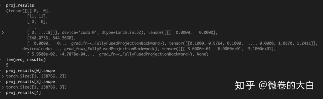
投影结果解析:
if packed:
    # packed模式:只返回可见的高斯,格式为 [nnz, ...]
    (
        batch_ids,      # batch索引
        camera_ids,     # 相机索引
        gaussian_ids,   # 高斯索引
        radii,          # 2D半径 [nnz, 2]
        means2d,        # 2D中心 [nnz, 2]
        depths,         # 深度值 [nnz]
        conics,         # 2D协方差逆矩阵 [nnz, 3]
        compensations,  # 抗锯齿补偿因子 [nnz]
    ) = proj_results
    # 根据可见性重新索引不透明度
    opacities = opacities.view(B, N)[batch_ids, gaussian_ids]
else:
    # 非packed模式:返回所有高斯,格式为 [C, N, ...]
    radii, means2d, depths, conics, compensations = proj_results
    # 广播不透明度到所有相机
    opacities = torch.broadcast_to(
        opacities[..., None, :], batch_dims + (C, N)
    )
    # radii(1, 138766, 2) , means2d (1, 138766, 2),  depths (1, 138766), conics (1, 138766, 2)

meta.update(
        {
            # global batch and camera ids
            "batch_ids": batch_ids,
            "camera_ids": camera_ids,
            # local gaussian_ids
            "gaussian_ids": gaussian_ids,
            "radii": radii,
            "means2d": means2d,
            "depths": depths,
            "conics": conics,
            "opacities": opacities,
        }
    )
球谐函数处理
if sh_degree is None:
    # 直接使用颜色值
    if packed:
        colors = colors.view(B, N, -1)[batch_ids, gaussian_ids]
    else:
        colors = torch.broadcast_to(
            colors[..., None, :, :], batch_dims + (C, N, -1)
        )
else:
    # 使用球谐函数计算视角相关的颜色
    # 1. 计算相机位置
    campos = torch.inverse(viewmats)[..., :3, 3]  # [C, 3]

    # 2. 计算视角方向(从高斯指向相机)
    if packed:
        dirs = (
            means.view(B, N, 3)[batch_ids, gaussian_ids]
            - campos.view(B, C, 3)[batch_ids, camera_ids]
        )  # [nnz, 3]
        masks = (radii > 0).all(dim=-1)  # 只计算可见高斯
    else:
        dirs = means[..., None, :, :] - campos[..., None, :]  # [C, N, 3]
        masks = (radii > 0).all(dim=-1)  # [C, N]

    # 3. 计算球谐函数
    colors = spherical_harmonics(
        sh_degree,  # 使用的SH阶数
        dirs,       # 视角方向
        shs,        # SH系数
        masks=masks # 跳过不可见的高斯
    )
    # colors(1, 138766, 3)

    # 4. 确保颜色非负
    colors = torch.clamp_min(colors + 0.5, 0.0)
tile 相交检测
# 计算tile 尺寸
tile_width = math.ceil(width / float(tile_size))   # 通常 tile_size=16
tile_height = math.ceil(height / float(tile_size))

# 找出每个高斯与哪些 tile 相交
tiles_per_gauss, isect_ids, flatten_ids = isect_tiles(
    means2d,        # 2D投影中心
    radii,          # 2D半径
    depths,         # 深度(用于排序)
    tile_size,      # tile大小(16x16)
    tile_width,     # 图片宽度方向有多少个 tile
    tile_height,    # 高度方向有多少个 tile
    segmented=segmented,
    packed=packed,
    n_images=I,
    image_ids=image_ids,
    gaussian_ids=gaussian_ids,
)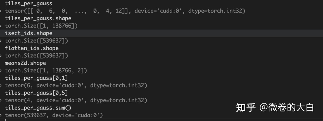
tiles_per_gauss:每个高斯球和多少个 tile 相交(会用于多少个 tile 的渲染,就需要 copy 多少份)
比如tiles_per_gauss[0, 5] = 4,表示第 5 个高斯球会用于 4 个图片tiles 的渲染
isect_ids : 记录 tile 与 image 关系
Shape为 需要参与渲染的高斯球数量(复制之后)如 debug 窗口所示,tiles_per_gauss.sum() = isect_ids.shape[-1]
其编码格式为:
# 64位整数编码了三个信息:
# |-- image_id --|-- tile_id --|-- depth (32bit) --|
# 高位                                          低位

# 提取tile_id(假设使用高位)
tile_bits = 16
tile_id = (1064392831 >> 16) & 0xFFFF  # = 16236

# 提取深度信息(低位)
depth_bits = 1064392831 & 0xFFFF  # = 9471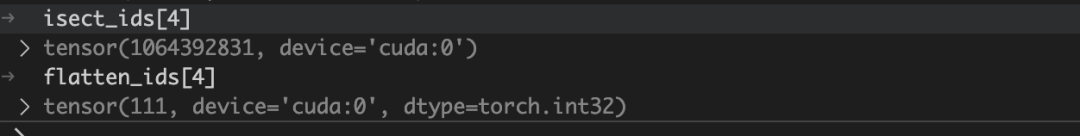
flatten_ids:表示第 i 个记录对应哪个高斯球
编码 offset 格式,并更新 meat
# 编码相交信息为偏移量(用于后续并行渲染时候快速索引)
isect_offsets = isect_offset_encode(
    isect_ids,      # 相交ID
    I,              # 图像总数
    tile_width,
    tile_height
)

isect_offsets = isect_offsets.reshape(batch_dims + (C, tile_height, tile_width))
# torch.Size([1, 53, 82])

meta.update(
    {
        "tile_width": tile_width,
        "tile_height": tile_height,
        "tiles_per_gauss": tiles_per_gauss,
        "isect_ids": isect_ids,
        "flatten_ids": flatten_ids,
        "isect_offsets": isect_offsets,
        "width": width,
        "height": height,
        "tile_size": tile_size,
        "n_batches": B,
        "n_cameras": C,
    }
)
光栅到像素
# 处理大通道数的情况(分块渲染)
if colors.shape[-1] > channel_chunk:  # channel_chunk=32
    n_chunks = (colors.shape[-1] + channel_chunk - 1) // channel_chunk
    render_colors, render_alphas = [], []

    for i in range(n_chunks):
        # 分块处理,避免显存溢出
        colors_chunk = colors[..., i * channel_chunk : (i + 1) * channel_chunk]

        render_colors_, render_alphas_ = rasterize_to_pixels(
            means2d,        # 2D中心
            conics,         # 2D协方差逆矩阵
            colors_chunk,   # 颜色块
            opacities,      # 不透明度
            width, height,
            tile_size,
            isect_offsets,  # 瓦片偏移
            flatten_ids,    # 展平索引
            backgrounds=backgrounds_chunk,
            packed=packed,
            absgrad=absgrad,  # 是否计算绝对梯度
        )
        render_colors.append(render_colors_)
        render_alphas.append(render_alphas_)

    render_colors = torch.cat(render_colors, dim=-1)
    render_alphas = render_alphas[0]
else:
    # 直接渲染
    render_colors, render_alphas = rasterize_to_pixels(
        means2d, conics, colors, opacities,
        width, height, tile_size,
        isect_offsets, flatten_ids,
        backgrounds=backgrounds,
        packed=packed,
        absgrad=absgrad,
    )
    # render_colors.shape :     torch.Size([1, 840, 1297, 3])
    # render_alphas.shape :    torch.Size([1, 840, 1297, 1])
返回
# 返回三个值
return (
    render_colors,  # 渲染的图像 [C, H, W, D]
    render_alphas,  # Alpha通道 [C, H, W, 1]
    meta           # 包含所有中间结果
)

meta = {
    'gaussian_ids': gaussian_ids,  # 参与渲染的高斯索引
    'radii': radii,               # 2D半径
    'means2d': means2d,           # 2D位置
    'depths': depths,             # 深度
    'conics': conics,             # 2D协方差逆
    'opacities': opacities,       # 不透明度
    'tiles_per_gauss': tiles_per_gauss,  # 瓦片覆盖数
    'isect_offsets': isect_offsets,      # 瓦片偏移
    # ... 更多调试信息
}
致密化策略
trian 循环调用 包括两部分
# 前向传播前:收集统计信息
self.cfg.strategy.step_pre_backward(
    params=self.splats,
    optimizers=self.optimizers,
    state=self.strategy_state,
    step=step,
    info=info,  # 包含梯度等信息
)

......

# 优化器更新后:执行实际的分裂/修剪
self.cfg.strategy.step_post_backward(
    params=self.splats,
    optimizers=self.optimizers,
    state=self.strategy_state,
    step=step,
    info=info,
    packed=cfg.packed,
)
更新策略:
def step_post_backward(
    self,
    params: Union[Dict[str, torch.nn.Parameter], torch.nn.ParameterDict],
    optimizers: Dict[str, torch.optim.Optimizer],
    state: Dict[str, Any],
    step: int,
    info: Dict[str, Any],
    packed: bool = False,
):
    """Callback function to be executed after the `loss.backward()` call."""
    if step >= self.refine_stop_iter:
        return

    self._update_state(params, state, info, packed=packed)

    if (
        step > self.refine_start_iter
        and step % self.refine_every == 0
        and step % self.reset_every >= self.pause_refine_after_reset
    ):
        # grow GSs
        n_dupli, n_split = self._grow_gs(params, optimizers, state, step)
        if self.verbose:
            print(
                f"Step {step}: {n_dupli} GSs duplicated, {n_split} GSs split. "
                f"Now having {len(params['means'])} GSs."
            )

        # prune GSs
        n_prune = self._prune_gs(params, optimizers, state, step)
        if self.verbose:
            print(
                f"Step {step}: {n_prune} GSs pruned. "
                f"Now having {len(params['means'])} GSs."
            )

        # reset running stats
        state["grad2d"].zero_()
        state["count"].zero_()
        if self.refine_scale2d_stop_iter > 0:
            state["radii"].zero_()
        torch.cuda.empty_cache()

    if step % self.reset_every == 0 and step > 0:
        reset_opa(
            params=params,
            optimizers=optimizers,
            state=state,
            value=self.prune_opa * 2.0,
        )
loss 计算
# loss
l1loss = F.l1_loss(colors, pixels)
ssimloss = 1.0 - fused_ssim(
    colors.permute(0, 3, 1, 2), pixels.permute(0, 3, 1, 2), padding="valid"
)
loss = l1loss * (1.0 - cfg.ssim_lambda) + ssimloss * cfg.ssim_lambda
if cfg.depth_loss:
    # query depths from depth map
    points = torch.stack(
        [
            points[:, :, 0] / (width - 1) * 2 - 1,
            points[:, :, 1] / (height - 1) * 2 - 1,
        ],
        dim=-1,
    )  # normalize to [-1, 1]
    grid = points.unsqueeze(2)  # [1, M, 1, 2]
    depths = F.grid_sample(
        depths.permute(0, 3, 1, 2), grid, align_corners=True
    )  # [1, 1, M, 1]
    depths = depths.squeeze(3).squeeze(1)  # [1, M]
    # calculate loss in disparity space
    disp = torch.where(depths > 0.0, 1.0 / depths, torch.zeros_like(depths))
    disp_gt = 1.0 / depths_gt  # [1, M]
    depthloss = F.l1_loss(disp, disp_gt) * self.scene_scale
    loss += depthloss * cfg.depth_lambda
if cfg.use_bilateral_grid:
    tvloss = 10 * total_variation_loss(self.bil_grids.grids)
    loss += tvloss

# regularizations
if cfg.opacity_reg > 0.0:
    loss += cfg.opacity_reg * torch.sigmoid(self.splats["opacities"]).mean()
if cfg.scale_reg > 0.0:
    loss += cfg.scale_reg * torch.exp(self.splats["scales"]).mean()

loss.backward()
多卡训练
是的,3dgs 的训练从去年开始就发展出了多种并行方式,用来加速训练和减少大场景的显存占用,gsplat 的并行实现来自 On Scaling Up 3D Gaussian Splatting Training ( On Scaling Up 3D Gaussian Splatting Training ) 作者提的 PR:https://github.com/nerfstudio-project/gsplat/pull/253 ,但是gsplat 的实现比Grendel 的开源实现少了像素负载均衡等功能。
并行方案的话,稍微有点像大模型里面的 TP + DSP 。
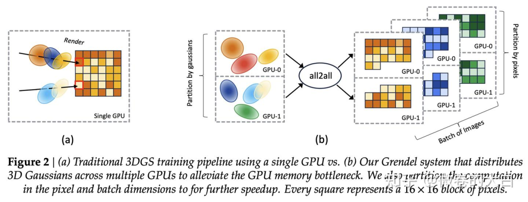
高斯球加载到不同的 GPU 上(类似 TP 切模型参数)
在 render 前,用 all_to_all / sparse_all_to_all 将高斯球并行转换为像素tile 渲染的并行(类似于 DSP 在多维 Transformer 间维度的转换)
在 loss 计算阶段,沿用像素块/图像间的并行。
这里简单过一下,如果感兴趣 gs 坑的人多,再展开吧。
高斯球切分
在初始化阶段切分,即create_splats_with_optimizers中:
# 将高斯球分配到不同的GPU
# points.shape : torch.Size([138766, 3])
points = points[world_rank::world_size]
# [rank1] points:  torch.Size([34692, 3])
rgbs = rgbs[world_rank::world_size]
scales = scales[world_rank::world_size]
统计通信所需参数
在 https://github.com/nerfstudio-project/gsplat/blob/main/gsplat/rendering.py# L360
# Implement the multi-GPU strategy proposed in
# `On Scaling Up 3D Gaussian Splatting Training <https://arxiv.org/abs/2406.18533>`.
#
# If in distributed mode, we distribute the projection computation over Gaussians
# and the rasterize computation over cameras. So first we gather the cameras
# from all ranks for projection.
if distributed:
    world_rank = torch.distributed.get_rank()  # 当前GPU编号
    world_size = torch.distributed.get_world_size()  # GPU总数

    # 1. 收集每个GPU上的高斯球数量
    # Gather the number of Gaussians in each rank.
    N_world = all_gather_int32(world_size, N, device=device)
    # N_world : [34692, 34692, 34691, 34691]

    # 2. 每个GPU负责相同数量的相机
    # Enforce that the number of cameras is the same across all ranks.
    C_world = [C] * world_size
    # [1, 1, 1, 1]

    # 3. 收集所有GPU的相机参数
    viewmats, Ks = all_gather_tensor_list(world_size, [viewmats, Ks])
    # viewmats.shape : torch.Size([4, 4, 4])
    # Ks.shape : torch.Size([4, 3, 3])
    # 现在每个GPU都有所有4个相机的参数

    # 4. 更新C为全局相机数
    C = len(viewmats)  # C从1变成4
Packed : sparse all_to_all
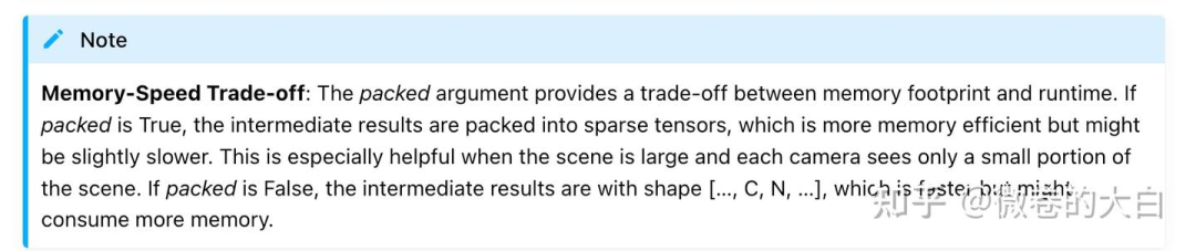
packed 说明可以参考:https://github.com/nerfstudio-project/gsplat/pull/253 和 https://docs.gsplat.studio/main/apis/rasterization.html
if packed:
    # 1. 统计每个相机看到多少高斯
    cnts = torch.bincount(camera_ids, minlength=C)

    # 2. 按GPU分组(每个GPU负责哪些相机)
    cnts = cnts.split(C_world, dim=0)
    cnts = [cuts.sum() for cuts in cnts] # 处理一个 rank 负责多个相机的情况
    # cnts [tensor(15987, device='cuda:1'), tensor(16784, device='cuda:1'), tensor(16449, device='cuda:1'), tensor(17097, device='cuda:1')]
    # 表示需要发送到各GPU的高斯数量

    # 3. All-to-All通信:
    # 统计不同rank 需要的高斯球数量 (是 2D projection 结果)
    collected_splits = all_to_all_int32(world_size, cnts, device=device)
    # collected_splits :[tensor(16804, device='cuda:1'), tensor(16784, device='cuda:1'), tensor(16917, device='cuda:1'), tensor(16700, device='cuda:1')]

    # 发送投影结果
    # all_to_all 前 , radii.shape :torch.Size([66317, 2])
    # 15987 + 16784 + 16449 + 17097 = 66317
    (radii,) = all_to_all_tensor_list(
        world_size, [radii], cnts, output_splits=collected_splits
    )
    # all_to_all 后, radii.shape :torch.Size([67205, 2])
    # 16804 + 16784 + 16917 + 16700 = 67205

    # all_to_all 前 , means2d.shape :torch.Size([66317, 2])
    (means2d, depths, conics, opacities, colors) = all_to_all_tensor_list(
        world_size,
        [means2d, depths, conics, opacities, colors],
        cnts,
        output_splits=collected_splits,
    )
    # # all_to_all 后, radii.shape :torch.Size([67205, 2])

    # 调整全局索引到 local 索引
    # before sending the data, we should turn the camera_ids from global to local.
    # i.e. the camera_ids produced by the projection stage are over all cameras world-wide,
    # so we need to turn them into camera_ids that are local to each rank.
    offsets = torch.tensor(
        [0] + C_world[:-1], device=camera_ids.device, dtype=camera_ids.dtype
    )# tensor([0, 1, 1, 1], device='cuda:1')
    offsets = torch.cumsum(offsets, dim=0)
    # offsets : tensor([0, 1, 2, 3], device='cuda:1')
    # cnts : [tensor(15987, device='cuda:1'), tensor(16784, device='cuda:1'), tensor(16449, device='cuda:1'), tensor(17097, device='cuda:1')]
    offsets = offsets.repeat_interleave(torch.stack(cnts))
    # tensor([0, 0, 0,  ..., 3, 3, 3], device='cuda:1')
    # offsets.shape : torch.Size([66317])
    # camera_ids : tensor([0, 0, 0,  ..., 3, 3, 3], device='cuda:1')
    camera_ids = camera_ids - offsets
    # camera_ids : tensor([0, 0, 0,  ..., 0, 0, 0], device='cuda:1')

    # and turn gaussian ids from local to global.
    offsets = torch.tensor(
        [0] + N_world[:-1],
        device=gaussian_ids.device,
        dtype=gaussian_ids.dtype,
    ) # tensor([    0, 34692, 34692, 34691], device='cuda:1')
    offsets = torch.cumsum(offsets, dim=0)
    offsets = offsets.repeat_interleave(torch.stack(cnts))
    # tensor([     0,      0,      0,  ..., 104075, 104075, 104075], device='cuda:1')
    # offsets.shape :torch.Size([66317])
    gaussian_ids = gaussian_ids + offsets

    # all to all communication across all ranks.
    # camera_ids.shape : torch.Size([66317])
    # gaussian_ids.shape : torch.Size([66317])
    (camera_ids, gaussian_ids) = all_to_all_tensor_list(
        world_size,
        [camera_ids, gaussian_ids],
        cnts,
        output_splits=collected_splits,
    )
    #  camera_ids.shape : torch.Size([67205])

    # Silently change C from global #Cameras to local #Cameras.
    C = C_world[world_rank]
非 packed :普通 all_to_all
不需要额外计算,全都通信,用的时候再加 mask
isect_tiles 和 rasterize_to_pixels 都也会包括 packed 参数
else:
    # 发送:每个GPU发送 C_i * N 个元素
    # 接收:每个GPU接收 C * N_i 个元素

    #radii.shape : torch.Size([4, 34692, 2])
    (radii,) = all_to_all_tensor_list(
        world_size,
        [radii.flatten(0, 1)],
        splits=[C_i * N for C_i in C_world],      # 发送大小
        output_splits=[C * N_i for N_i in N_world], # 接收大小
    )
    # #radii.shape : torch.Size([138776, 2])

    # 按相机数量 reshpae
    radii = reshape_view(C, radii, N_world)
    # torch.Size([1, 138766, 2])

    (means2d, depths, conics, opacities, colors) = all_to_all_tensor_list(
        world_size,
        [
            means2d.flatten(0, 1),
            depths.flatten(0, 1),
            conics.flatten(0, 1),
            opacities.flatten(0, 1),
            colors.flatten(0, 1),
        ],
        splits=[C_i * N for C_i in C_world],
        output_splits=[C * N_i for N_i in N_world],
    )
    means2d = reshape_view(C, means2d, N_world)
    depths = reshape_view(C, depths, N_world)
    conics = reshape_view(C, conics, N_world)
    opacities = reshape_view(C, opacities, N_world)
    colors = reshape_view(C, colors, N_world)
自动驾驶之心
论文辅导来啦

自驾交流群来啦!
自动驾驶之心创建了近百个技术交流群,涉及大模型、VLA、端到端、数据闭环、自动标注、BEV、Occupancy、多模态融合感知、传感器标定、3DGS、世界模型、在线地图、轨迹预测、规划控制等方向!欢迎添加小助理微信邀请进群。

知识星球交流社区
近4000人的交流社区,近300+自动驾驶公司与科研结构加入!涉及30+自动驾驶技术栈学习路线,从0到一带你入门自动驾驶感知(大模型、端到端自动驾驶、世界模型、仿真闭环、3D检测、车道线、BEV感知、Occupancy、多传感器融合、多传感器标定、目标跟踪)、自动驾驶定位建图(SLAM、高精地图、局部在线地图)、自动驾驶规划控制/轨迹预测等领域技术方案、大模型,更有行业动态和岗位发布!欢迎加入。

独家专业课程
端到端自动驾驶、大模型、VLA、仿真测试、自动驾驶C++、BEV感知、BEV模型部署、BEV目标跟踪、毫米波雷达视觉融合、多传感器标定、多传感器融合、多模态3D目标检测、车道线检测、轨迹预测、在线高精地图、世界模型、点云3D目标检测、目标跟踪、Occupancy、CUDA与TensorRT模型部署、大模型与自动驾驶、NeRF、语义分割、自动驾驶仿真、传感器部署、决策规划、轨迹预测等多个方向学习视频
学习官网:www.zdjszx.com


 918
918

 被折叠的 条评论
为什么被折叠?
被折叠的 条评论
为什么被折叠?
 到【灌水乐园】发言


