机器人逆运动学——以六自由度机器人为例（详解、易懂，附全部Matlab代码）

六自由度机器人逆运动学解析

原创于 2025-10-12 21:08:25 发布 · 1.6k 阅读

33 ·

CC 4.0 BY-SA版权

文章标签：

#机器人

机器人学-学习笔记专栏收录该内容

14 篇文章

订阅专栏

前言

前面机器人正运动学主要讲关节变量到末端执行器位姿的关系，也就是知道了关节变量与连杆参数就可以利用D-H参数表来表达末端位姿。而逆运动学就是已知末端的位姿与连杆参数，来求得关节变量的过程。本文首先介绍何为逆运动学，再以例子的形式利用D-H参数表与齐次变换矩阵对机器人进行逆解。

**阅读提醒1：在运动学逆解前，需要掌握运动学正解的相关知识，也要掌握一定的矩阵运算规则。（相关知识点有在我之前的文章提到，我也在本文进行了引用，如有需要可以查阅；我对机器人正运动学相关的matlab分析单独发了一篇博客，有需要也可以查阅）

**阅读提醒2：下文灰色补充块是用于解释正文的，用来补充正文没讲到的知识或细节。

一、运动学逆解

上面提到，已知末端执行器的位姿来求解这一位姿对应的全部关节变量就是逆解，然而由于机械结构的差异，有些时候一个末端位姿可能对应着不同的反解情况(多解)。逆运动学问题实质就是非线性超越方程组的求解问题，其解法分为两大类（封闭解法和数值解法），本文主要讲封闭解法。

1.【封闭解法】概述

封闭解法是指具有解析形式的解法，其计算速度快、效率高，更便于实时控制，具体又可以分为代数解法和几何解法。Pieper准则是机械臂存在封闭逆解的充分条件，并且满足其一即可，具体内容为：

Pieper准则：

1. 三个相邻关节轴相交于一点；

2. 三个相邻关节轴相互平行。

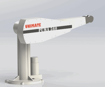
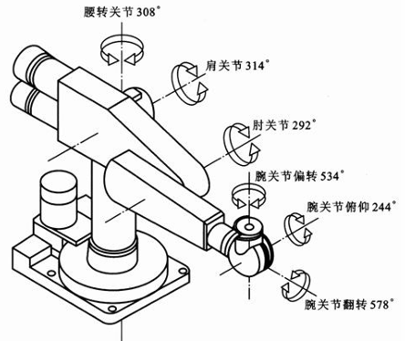
为简化逆解运算，如今机械臂厂家的大多机械臂结构都满足这一准则，比如下面常见的PUMA560机械臂(6R机械臂)，属于关节式机器人，一共有6个关节且都是转动关节，前3个关节确定手腕参考点的位置，后3个关节确定手腕的方位：

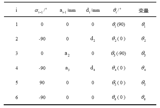
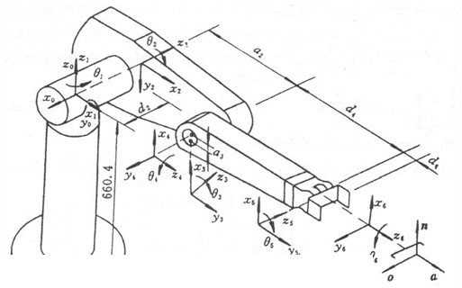
为了方便写下面的逆变换求解，先把该机器人对应的D-H参数表列在下方（具体得到过程之前有写）：

2. 逆解具体过程（代数详解）

PUMA560六自由度机器人的2、3、4关节轴平行，所以满足Pieper准则，运用封闭解法来对其进行运动学逆解如下：

首先先列写其一般变换方程如下式（要知道 $_{6}^{0}\textrm{}T$ 可以通过连杆参数等，一步步乘出结果）：

$_{6}^{0}\textrm{}T=\begin{bmatrix} n_{x} & o_{x} & a_{x} & p_{x}\\ n_{y} & o_{y} & a_{y} &p_{y} \\ n_{z} & o_{z} & a_{z} &p_{z} \\ 0 & 0& 0& 1 \end{bmatrix}=_{1}^{0}\textrm{}T\left ( \theta _{1} \right )_{2}^{1}\textrm{}T\left ( \theta _{2} \right )_{3}^{2}\textrm{}T\left ( \theta _{3} \right )_{4}^{3}\textrm{}T\left ( \theta _{4} \right )_{5}^{4}\textrm{}T\left ( \theta _{5} \right )_{6}^{5}\textrm{}T\left ( \theta _{6} \right )$

末端执行器的位姿为 $\vec{n}$ 、 $\vec{o}$ 、 $\vec{a}$ 、 $\vec{p}$ ，问题也就转变为知道这些参量，来求解 $\theta$ 这6个关节变量。过程就是用未知的连杆逆变换来左乘上式的等号两边，这样就能把关节变量分离出来，进而就能求解，具体如下：

① $\theta _{1}$ 求解

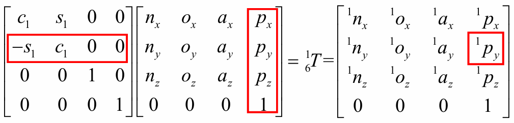
将一般变换方程两端左乘 $_{1}^{0}\textrm{}T^{-1}\left (\theta _{1} \right )$ 得到下式，这样左侧就分离出只有 $\theta _{1}$ 的变量：

$_{1}^{0}\textrm{}T^{-1}\left (\theta _{1} \right )_{6}^{0}\textrm{}T=_{2}^{1}\textrm{}T\left ( \theta _{2} \right )_{3}^{2}\textrm{}T\left ( \theta _{3} \right )_{4}^{3}\textrm{}T\left ( \theta _{4} \right )_{5}^{4}\textrm{}T\left ( \theta _{5} \right )_{6}^{5}\textrm{}T\left ( \theta _{6} \right )$

补充：如何求 $_{1}^{0}\textrm{}T^{-1}\left (\theta _{1} \right )$ ？

我们已知齐次变换矩阵实际是由旋转矩阵与平移向量的复合也就是：

$_{B}^{A}\textrm{}T=\begin{bmatrix} _{B}^{A}\textrm{}R & ^{A}\textrm{}P_{B_{0}}\\ 0 00 & 1 \end{bmatrix}$

套用公式，其实际上变换矩阵的逆矩阵为：

$_{B}^{A}\textrm{}T^{-1}=\begin{bmatrix} _{B}^{A}\textrm{}R^{-1} & -_{B}^{A}\textrm{}R^{-1}\textrm{}P_{B_{0}} \\ 0 00 & 1 \end{bmatrix}=\begin{bmatrix} _{B}^{A}\textrm{}R^{T} & -_{B}^{A}\textrm{}R^{T}\textrm{}P_{B_{0}} \\ 0 00 & 1 \end{bmatrix}$

也就是齐次变换矩阵求逆：让对应的旋转矩阵处求逆（也就是转置），位移列向量处左乘一个负的旋转矩阵的逆（转置）。

*（ $_{6}^{0}\textrm{}T$ 在之前的文章中已经用Matlab求过了，可以再回头看一下。）

结合上面补充分析，等号左右两式矩阵可得下式：

具体计算过程：

想要逆解出变量结果，就需要真正算出左侧两矩阵相乘后的结果（主要是为了得到 $^{1}\textrm{}p_{x}$ 、 $^{1}\textrm{}p_{y}$ 、 $^{1}\textrm{}p_{z}$ ），这里我用Matlab确实具体算了一遍，结果如下：

①首先先算一下 $p_{x}$ 、 $p_{y}$ 和 $p_{z}$ 的值：

$p_{x}=c_1\left [ a_2c_2-d_4s_{23}+a_3c_{23} \right ]-d_2s_1$

$p_{y}=s_1\left [ a_2c_2+a_3c_{23}-d_4s_{23} \right ]+d_2c_1$

$p_{z}=-\left [ a_3s_{23}+d_4c_{23}-a_2s_{2} \right ]$

以上是用齐次变换矩阵定义，利用matlab计算出的。

--------------------------------------------------------------------------------------------------------------------

②所以计算上面式等号左边两红框相乘的结果：

$-s_1p_{x}+c_1p_y=-s_1\left \{ c_1\left [ a_2c_2-d_4s_{23}+a_3c_{23} \right ]-d_2s_1 \right \}+c_1\left \{ s_1\left [ a_2c_2+a_3c_{23}-d_4s_{23} \right ]+d_2c_1 \right \}=d_2\left ( c_{1}^{2} + s_{1}^{2}\right )=d_2$

这一步就是按部就班代入、乘开这个式子，然后合并消除后就只剩下 $d_2$ 了，不要被大长式子吓到。

所以可以得到： $^{1}\textrm{}p_{y}=d_{2}$

--------------------------------------------------------------------------------------------------------------------

③同理也可以去计算矩阵两端（1，4）和（3，4）的元素：

$^{1}\textrm{}p_{x}=c_1p_{x}+s_1p_y=c_1\left \{ c_1\left [ a_2c_2-d_4s_{23}+a_3c_{23} \right ]-d_2s_1 \right \}+s_1\left \{ s_1\left [ a_2c_2+a_3c_{23}-d_4s_{23} \right ]+d_2c_1 \right \}=a_2c_2+a_3c_{23}-d_4s_{23}$

$^{1}\textrm{}p_{z}=p_{z}=-\left [ a_3s_{23}+d_4c_{23}-a_2s_{2} \right ]$

*( $c_{1}$ 就是 $cos\theta _{1}$ ， $s_{1}$ 就是 $sin\theta _{1}$ ， $c_{23}$ 就是 $cos\left ( \theta _{2}+\theta _{3} \right )$ ， $s_{23}$ 就是 $sin\left ( \theta _{2}+\theta _{3} \right )$ ，这里不赘述。)

式中： $^{1}\textrm{}p_{y}=d_{2}$

之后令等号两端的（2，4）元素相等（红框已经圈出）：

补充：三角代换知识。如何求 $acos\theta +bsin\theta =c$ 中的 $\theta$ ？

解：利用中间变量进行变换

其中 $tan\left ( \frac{\theta }{2} \right )=u$ ， $cos\theta =\frac{1-u^{2}}{1+u^{2}}$ ， $sin\theta =\frac{2u}{1+u^{2}}$

所以：

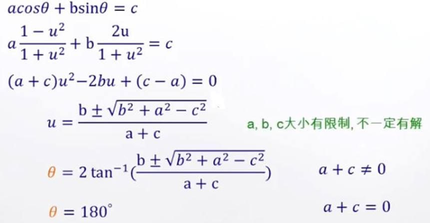
通过三角代换： $p_{x}=\rho cos\phi$ ， $p_{y}=\rho sin\phi$ 。其中 $\rho =\sqrt{p_{x}^{2}+p_{y}^{2}}$ ， $\phi =Atan2\left ( p_{x}, p_{y}\right )$ 。

代入后得到：

$\theta_1 = \text{Atan2}(p_y, p_x) - \text{Atan2}\left(d_2, \pm \sqrt{p_x^2 + p_y^2 - d_2^2}\right)$

式中，正负号代表了 $\theta _{1}$ 的两个可能解。

② $\theta _{3}$ 求解

选定 $\theta _{1}$ 一个解之后，再令 $_{6}^{1}\textrm{}T$ 两端元素（1，4）与（3，4）分别相等，可以得到下面方程组：

$\left\{ \begin{aligned} c_1 p_x + s_1 p_y &= a_3 c_{23} - d_4 s_{23} + a_2 c_2 \\ p_z &= -\left [ a_3s_{23}+d_4c_{23}-a_2s_{2} \right ] \end{aligned} \right.$

之后让 $-s_1p_x+c_1p_y=d_2$ 与此方程组平方求和，可以得到：

$a_3c_3-d_4s_3=k$

式中， $k = \frac{p_x^2 + p_y^2 + p_z^2 - a_2^2 - a_3^2 - d_2^2 - d_4^2}{2 a_2 }$

这样就可以实现式中只有一个变量 $\theta _{3}$ ，并且这个等式形式和上面求 $\theta _{1}$ 时一致，所以同理：

$\theta_3 = \text{Atan2}(a_3, d_4) - \text{Atan2}\left(k, \pm \sqrt{a_3^2 + d_4^2 - k^2}\right)$

式中，正负号代表了 $\theta _{3}$ 的两个可能解。

③ $\theta _{2}$ 求解

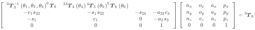
将一般变换方程等式两边左乘一个 $_{3}^{0}\textrm{}T^{-1}\left (\theta _{1}, \theta _{2} ,\theta _{3} \right )$ ，如下：

$_{3}^{0}\textrm{}T^{-1}\left (\theta _{1} ,\theta _{2},\theta _{3}\right )_{6}^{0}\textrm{}T=_{4}^{3}\textrm{}T\left ( \theta _{4} \right )_{5}^{4}\textrm{}T\left ( \theta _{5} \right )_{6}^{5}\textrm{}T\left ( \theta _{6} \right )$

这样就可以使得等号左侧只有三个变量，而前面求了 $\theta _{1}$ 与 $\theta _{3}$ ，因此就只有 $\theta _{2}$ 这一个变量了。等号左右两式矩阵可得下式：

通过计算可以得到 $^{_{3}^{0}\textrm{}}T$ ：

$^{_{3}^{0}\textrm{}}T=\begin{bmatrix} c_1c_{23} & -c_{1} s_{23} & -s_1&a_2c_1c_2-d_2s_1 \\ s_1c_{23} & -s_1s_{23} & c_1 & d_2c_1+a_2c_2s_1\\ -s_{23} & -c_{23} & 0&-a_2s_2 \\ 0& 0 & 0 &1 \end{bmatrix}$

然后再根据矩阵求逆的方法去计算 $^{_{3}^{0}\textrm{}}T^{-1}$ ，这里不再赘述~

上式中等号左边的矩阵就是计算后的 $^{_{3}^{0}\textrm{}}T^{-1}$ (这里简化表达)，然后令上式的（1，4）与（2，4）元素相等进行计算，最后合并消除可以得到：

$\theta_{23} = \theta_2 + \theta_3 = \text{atan2}\left[ -(a_3 + a_2 c_3) p_z + (c_1 p_x + s_1 p_y)(a_2 s_3 - d_4), (-d_4 + a_2 s_3) p_x + (c_1 p_x + s_1 p_y)(a_2 c_3 + a_3) \right]$

$\theta _{2}=\theta _{23}-\theta _{3}$

其中 $\theta _{3}$ 的解与 $\theta _{1}$ 和 $\theta _{2}$ 有关，因此得出的 $\theta _{3}$ 有四种可能的解。

④ $\theta _{4}$ 求解

因为上面 $_{6}^{3}\textrm{}T$ 左式均为已知，令两边的元素（1，3）和（3，3）分别相等，则可以得到：

$\left\{ \begin{aligned} a_x c_{1} c_{23} + a_y s_{1} c_{23} - a_z s_{23} &= -c_4 s_5 \\ -a_x s_y + a_y c_1 &= s_4 s_5 \end{aligned} \right.$

这里面只要 $s_{5}$ 不为0，消去之后就可以得到 $\theta _{4}$ ：

$\theta_4 = \text{Atan2}\left( -a_4 s_1 + a_y c_1, -a_x c_1 c_{23} - a_y s_1 c_{23} + a_z s_{23} \right)$

如果 $s_{5}=0$ ，此时机械臂处于奇异位置，这时候关节4与6重合，不能解出来具体值，这个奇异值我们后面讨论。

⑤ $\theta _{5}$ 求解

可以让一般变换方程等式两边左乘一个 $_{4}^{0}\textrm{}T^{-1}\left (\theta _{1}, \theta _{2} ,\theta _{3} , \theta _{4} \right )$ ，如下：

$_{4}^{0}\textrm{}T^{-1}\left (\theta _{1} ,\theta _{2},\theta _{3} ,\theta _{4} \right )_{6}^{0}\textrm{}T= _{5}^{4}\textrm{}T\left ( \theta _{5} \right )_{6}^{5}\textrm{}T\left ( \theta _{6} \right )$

这时候前面四个变量都解出来了，所以左侧只有 $\theta _{5}$ 一个变量未知。因此可以求出 $_{4}^{0}\textrm{}T^{-1}\left (\theta _{1}, \theta _{2} ,\theta _{3} , \theta _{4} \right )$ 矩阵：

$\left[ \begin{array}{cccc} c_1 c_{23} c_4 + s_1 s_4 & s_1 c_{23} c_4 - c_1 s_4 & -s_{23} c_4 & -a_2 c_3 c_4 + d_2 s_4 - a_3 c_4 \\ -c_1 c_{23} s_4 + s_1 c_4 & -s_1 c_{23} s_4 - c_1 c_4 & s_{23} s_4 & a_2 c_3 s_4 + d_2 c_4 + a_3 s_4 \\ -c_1 s_{23} & -s_1 s_{23} & -c_{23} & a_2 s_3 - d_4 \\ 0 & 0 & 0 & 1 \end{array} \right]$

同理，可以让等式两侧元素（1，3）和（3，3）分别相等，可以得到：

$\left\{ \begin{aligned} a_x \left( c_1 c_{23} c_4 + s_1 s_4 \right) + a_y \left( s_1 c_{23} c_4 - c_1 s_4 \right) - a_z \left( s_{23} c_4 \right) &= -s_5 \\ a_x \left( -c_1 s_{23} \right) + a_y \left( -s_1 s_{23} \right) + a_z \left( -c_{23} \right) &= c_5 \end{aligned} \right.$

由此得到 $\theta _{5}$ ：

$\theta _5=Atan2\left ( s_5, c_5 \right )$

⑥ $\theta _{6}$ 求解

同理让一般变换方程等式两边左乘一个 $_{5}^{0}\textrm{}T^{-1}\left (\theta _{1}, \theta _{2} ,\theta _{3} , \theta _{4} , \theta _{5} \right )$ ，如下：

$_{5}^{0}\textrm{}T^{-1}\left (\theta _{1} ,\theta _{2},\theta _{3} ,\theta _{4} , \theta _{5} \right )_{6}^{0}\textrm{}T= _{6}^{5}\textrm{}T\left ( \theta _{6} \right )$

通过上面等式（3，1）与（1，1）的元素相等，可以得到 $\theta _{6}$ ：

$\begin{cases} -n_x \left( c_1 c_{23} s_4 - s_1 c_4 \right) - n_y \left( s_1 c_{23} s_4 + c_1 c_4 \right) + n_z \left( s_{23} s_4 \right) = s_6 \\ n_x \left[ \left( c_1 c_{23} c_4 + s_1 s_4 \right) c_5 - c s_{23} s_5 \right] + n_y \left[ \left( s_1 c_{23} c_4 - c_1 s_4 \right) c_5 - s_1 s_{23} s_5 \right] - n_z \left( s_{23} c_4 c_5 + c_{23} s_5 \right) = c_6 \end{cases}$

$\theta _6=Atan2\left ( s_6, c_6 \right )$

至此六个变量求解完成，以上存在多解的关节还需要考虑关节结构，是否能够到达这一位置，如果因结构限制则可能这对应的解不存在。

二、Matlab求解过程

1. 整体代码

先把具体代码展示如下：

clc;
clear;

%输入已知的位姿矩阵（正解可得）----------------------
a=[ 0.0000    0.0000    1.0000  800.0000;
   -0.0000   -1.0000    0.0000  120.0000;
    1.0000   -0.0000   -0.0000   10.0000;
         0         0         0    1.0000 ];
%-------------------------------------------------

%定义连杆的D-H参数
%连杆偏移
d1 = 0; d2 = 120; d3 = 0; d4 = 400; d5 = 0; d6 = 0;
%连杆长度
a2 = 400; a3 = 10;
%连杆扭角
alpha1 = 0; alpha2 = -pi/2; alpha3 = 0; alpha4 = -pi/2; alpha5 = pi/2; alpha6 = -pi/2;
%建立机器人模型
%       theta  d        a        alpha     
L1=Link([0     d1       0        alpha1     ],'modified');
L2=Link([0     d2       0        alpha2     ],'modified');
L3=Link([0     d3       a2       alpha3     ],'modified');
L4=Link([0     d4       a3       alpha4     ],'modified');
L5=Link([0     d5       0        alpha5     ],'modified');
L6=Link([0     d6       0        alpha6     ],'modified');
%限制关节空间
L1.qlim = [(-165/180)*pi,(165/180)*pi];
L2.qlim = [(-150/180)*pi, (60/180)*pi];
L3.qlim = [(-150/180)*pi, (90/180)*pi];
L4.qlim = [(-180/180)*pi,(180/180)*pi];
L5.qlim = [(-115/180)*pi,(115/180)*pi];
L6.qlim = [(-360/180)*pi,(360/180)*pi];
%连接连杆，机器人取名为robot
robot=SerialLink([L1 L2 L3 L4 L5 L6],'name','6Rrobot');
robot.display();                    
robot.teach();                     

nx=a(1,1);ox=a(1,2);ax=a(1,3);px=a(1,4);
ny=a(2,1);oy=a(2,2);ay=a(2,3);py=a(2,4);
nz=a(3,1);oz=a(3,2);az=a(3,3);pz=a(3,4);

%解关节1
theta1_1 = atan2(py,px)-atan2(d2,abs(sqrt(px^2+py^2-d2^2)));
theta1_2 = atan2(py,px)-atan2(d2,-abs(sqrt(px^2+py^2-d2^2)));

%解关节3  kk为中间值
kk = (px^2+py^2+pz^2-a2^2-a3^2-d2^2-d4^2)/(2*a2);
theta3_1 = atan2(a3,d4)-atan2(kk,abs(sqrt(a3^2+d4^2-kk^2)));
theta3_2 = atan2(a3,d4)-atan2(kk,-abs(sqrt(a3^2+d4^2-kk^2)));

%解关节2  ko2为theta23计算式中第一部分,kt2为第二部分
% theta1_1 theta3_1对应解
ko2_1 = -((a3+a2*cos(theta3_1))*pz)+(cos(theta1_1)*px+sin(theta1_1)*py)*(a2*sin(theta3_1)-d4);
kt2_1 = (-d4+a2*sin(theta3_1))*pz+(cos(theta1_1)*px+sin(theta1_1)*py)*(a2*cos(theta3_1)+a3);
theta23_1 = atan2(ko2_1,kt2_1);
theta2_1 = theta23_1 - theta3_1;
% theta1_2 theta3_1对应解
ko2_2 = -((a3+a2*cos(theta3_1))*pz)+(cos(theta1_2)*px+sin(theta1_2)*py)*(a2*sin(theta3_1)-d4);
kt2_2 = (-d4+a2*sin(theta3_1))*pz+(cos(theta1_2)*px+sin(theta1_2)*py)*(a2*cos(theta3_1)+a3);
theta23_2 = atan2(ko2_2,kt2_2);
theta2_2 = theta23_2 - theta3_1;
% theta1_1 theta3_2对应解 
ko2_3 = -((a3+a2*cos(theta3_2))*pz)+(cos(theta1_1)*px+sin(theta1_1)*py)*(a2*sin(theta3_2)-d4);
kt2_3 = (-d4+a2*sin(theta3_2))*pz+(cos(theta1_1)*px+sin(theta1_1)*py)*(a2*cos(theta3_2)+a3);
theta23_3 = atan2(ko2_3,kt2_3);
theta2_3 = theta23_3 - theta3_2;
% theta1_2 theta3_2对应解 
ko2_4 = -((a3+a2*cos(theta3_2))*pz)+(cos(theta1_2)*px+sin(theta1_2)*py)*(a2*sin(theta3_2)-d4);
kt2_4 = (-d4+a2*sin(theta3_2))*pz+(cos(theta1_2)*px+sin(theta1_2)*py)*(a2*cos(theta3_2)+a3);
theta23_4 = atan2(ko2_4,kt2_4);
theta2_4 = theta23_4 - theta3_2;

% 求解关节4
% theta1_1 theta2_1  theta3_1对应解
ko4_1=-ax*sin(theta1_1)+ay*cos(theta1_1);
kt4_1=-ax*cos(theta1_1)*cos(theta23_1)-ay*sin(theta1_1)*cos(theta23_1)+az*sin(theta23_1);
theta4_1=atan2(ko4_1,kt4_1);
% theta1_2 theta2_2  theta3_1对应解
ko4_2=-ax*sin(theta1_2)+ay*cos(theta1_2);
kt4_2=-ax*cos(theta1_2)*cos(theta23_2)-ay*sin(theta1_2)*cos(theta23_2)+az*sin(theta23_2);
theta4_2=atan2(ko4_2,kt4_2);
% theta1_1 theta2_3  theta3_2对应解
ko4_3=-ax*sin(theta1_1)+ay*cos(theta1_1);
kt4_3=-ax*cos(theta1_1)*cos(theta23_3)-ay*sin(theta1_1)*cos(theta23_3)+az*sin(theta23_3);
theta4_3=atan2(ko4_3,kt4_3);
% theta1_2 theta2_4  theta3_2对应解
ko4_4=-ax*sin(theta1_2)+ay*cos(theta1_2);
kt4_4=-ax*cos(theta1_2)*cos(theta23_4)-ay*sin(theta1_2)*cos(theta23_4)+az*sin(theta23_4);
theta4_4=atan2(ko4_4,kt4_4);

% 求解关节5
% theta1_1 theta2_1  theta3_1 theta4_1 对应解
ko5_1=-ax*(cos(theta1_1)*cos(theta23_1)*cos(theta4_1)+sin(theta1_1)*sin(theta4_1))-ay*(sin(theta1_1)*cos(theta23_1)*cos(theta4_1)-cos(theta1_1)*sin(theta4_1))+az*(sin(theta23_1)*cos(theta4_1));
kt5_1= ax*(-cos(theta1_1)*sin(theta23_1))+ay*(-sin(theta1_1)*sin(theta23_1))+az*(-cos(theta23_1));
theta5_1=atan2(ko5_1,kt5_1);
% theta1_2 theta2_2  theta3_1 theta4_2 对应解
ko5_2=-ax*(cos(theta1_2)*cos(theta23_2)*cos(theta4_2)+sin(theta1_2)*sin(theta4_2))-ay*(sin(theta1_2)*cos(theta23_2)*cos(theta4_2)-cos(theta1_2)*sin(theta4_2))+az*(sin(theta23_2)*cos(theta4_2));
kt5_2= ax*(-cos(theta1_2)*sin(theta23_2))+ay*(-sin(theta1_2)*sin(theta23_2))+az*(-cos(theta23_2));
theta5_2=atan2(ko5_2,kt5_2);
% theta1_1 theta2_3  theta3_2 theta4_3 对应解
ko5_3=-ax*(cos(theta1_1)*cos(theta23_3)*cos(theta4_3)+sin(theta1_1)*sin(theta4_3))-ay*(sin(theta1_1)*cos(theta23_3)*cos(theta4_3)-cos(theta1_1)*sin(theta4_3))+az*(sin(theta23_3)*cos(theta4_3));
kt5_3= ax*(-cos(theta1_1)*sin(theta23_3))+ay*(-sin(theta1_1)*sin(theta23_3))+az*(-cos(theta23_3));
theta5_3=atan2(ko5_3,kt5_3);
% theta1_2 theta2_4  theta3_2 theta4_4 对应解
ko5_4=-ax*(cos(theta1_2)*cos(theta23_4)*cos(theta4_4)+sin(theta1_2)*sin(theta4_4))-ay*(sin(theta1_2)*cos(theta23_4)*cos(theta4_4)-cos(theta1_2)*sin(theta4_4))+az*(sin(theta23_4)*cos(theta4_4));
kt5_4= ax*(-cos(theta1_2)*sin(theta23_4))+ay*(-sin(theta1_2)*sin(theta23_4))+az*(-cos(theta23_4));
theta5_4=atan2(ko5_4,kt5_4);

% 求解关节角6
%  theta1_1 theta2_1  theta3_1 theta4_1  theta5_1 对应解
ko6_1=-nx*(cos(theta1_1)*cos(theta23_1)*sin(theta4_1)-sin(theta1_1)*cos(theta4_1))-ny*(sin(theta1_1)*cos(theta23_1)*sin(theta4_1)+cos(theta1_1)*cos(theta4_1))+nz*(sin(theta23_1)*sin(theta4_1));
kt6_1= nx*(cos(theta1_1)*cos(theta23_1)*cos(theta4_1)+sin(theta1_1)*sin(theta4_1))*cos(theta5_1)-nx*cos(theta1_1)*sin(theta23_1)*sin(theta4_1)+ny*(sin(theta1_1)*cos(theta23_1)*cos(theta4_1)+cos(theta1_1)*sin(theta4_1))*cos(theta5_1)-ny*sin(theta1_1)*sin(theta23_1)*sin(theta5_1)-nz*(sin(theta23_1)*cos(theta4_1)*cos(theta5_1)+cos(theta23_1)*sin(theta5_1));
theta6_1=atan2(ko6_1,kt6_1);
%  theta1_2 theta2_2  theta3_1 theta4_2  theta5_2 对应解
ko6_2=-nx*(cos(theta1_2)*cos(theta23_2)*sin(theta4_2)-sin(theta1_2)*cos(theta4_2))-ny*(sin(theta1_2)*cos(theta23_2)*sin(theta4_2)+cos(theta1_2)*cos(theta4_2))+nz*(sin(theta23_2)*sin(theta4_2));
kt6_2= nx*(cos(theta1_2)*cos(theta23_2)*cos(theta4_2)+sin(theta1_2)*sin(theta4_2))*cos(theta5_2)-nx*cos(theta1_2)*sin(theta23_2)*sin(theta4_2)+ny*(sin(theta1_2)*cos(theta23_2)*cos(theta4_2)+cos(theta1_2)*sin(theta4_2))*cos(theta5_2)-ny*sin(theta1_2)*sin(theta23_2)*sin(theta5_2)-nz*(sin(theta23_2)*cos(theta4_2)*cos(theta5_2)+cos(theta23_2)*sin(theta5_2));
theta6_2=atan2(ko6_2,kt6_2);
%  theta1_1 theta2_3  theta3_2 theta4_3  theta5_3 对应解
ko6_3=-nx*(cos(theta1_1)*cos(theta23_3)*sin(theta4_3)-sin(theta1_1)*cos(theta4_3))-ny*(sin(theta1_1)*cos(theta23_3)*sin(theta4_3)+cos(theta1_1)*cos(theta4_3))+nz*(sin(theta23_3)*sin(theta4_3));
kt6_3= nx*(cos(theta1_1)*cos(theta23_3)*cos(theta4_3)+sin(theta1_1)*sin(theta4_3))*cos(theta5_3)-nx*cos(theta1_1)*sin(theta23_3)*sin(theta4_3)+ny*(sin(theta1_1)*cos(theta23_3)*cos(theta4_3)+cos(theta1_1)*sin(theta4_3))*cos(theta5_3)-ny*sin(theta1_1)*sin(theta23_3)*sin(theta5_3)-nz*(sin(theta23_3)*cos(theta4_3)*cos(theta5_3)+cos(theta23_3)*sin(theta5_3));
theta6_3=atan2(ko6_3,kt6_3);
%  theta1_2 theta2_4  theta3_2 theta4_4  theta5_4 对应解
ko6_4=-nx*(cos(theta1_2)*cos(theta23_4)*sin(theta4_4)-sin(theta1_2)*cos(theta4_4))-ny*(sin(theta1_1)*cos(theta23_4)*sin(theta4_4)+cos(theta1_2)*cos(theta4_4))+nz*(sin(theta23_4)*sin(theta4_4));
kt6_4= nx*(cos(theta1_2)*cos(theta23_4)*cos(theta4_4)+sin(theta1_2)*sin(theta4_4))*cos(theta5_4)-nx*cos(theta1_2)*sin(theta23_4)*sin(theta4_4)+ny*(sin(theta1_2)*cos(theta23_4)*cos(theta4_4)+cos(theta1_2)*sin(theta4_4))*cos(theta5_1)-ny*sin(theta1_2)*sin(theta23_4)*sin(theta5_4)-nz*(sin(theta23_4)*cos(theta4_4)*cos(theta5_4)+cos(theta23_4)*sin(theta5_4));
theta6_4=atan2(ko6_4,kt6_4);

% 整理得到4组运动学非奇异逆解
theta_MOD1 = [ 
               theta1_1,theta2_1,theta3_1,theta4_1,theta5_1,theta6_1;
 			   theta1_2,theta2_2,theta3_1,theta4_2,theta5_2,theta6_2;
 			   theta1_1,theta2_3,theta3_2,theta4_3,theta5_3,theta6_3;
 			   theta1_2,theta2_4,theta3_2,theta4_4,theta5_4,theta6_4;
              ]*(180/pi);
% 将操作关节‘翻转’可得到另外4组解
theta_MOD2 = ...
    [ 
      theta1_1,theta2_1,theta3_1,theta4_1+pi,-theta5_1,theta6_1+pi;
 	  theta1_2,theta2_2,theta3_1,theta4_2+pi,-theta5_2,theta6_2+pi;
 	  theta1_1,theta2_3,theta3_2,theta4_3+pi,-theta5_3,theta6_3+pi;
 	  theta1_2,theta2_4,theta3_2,theta4_4+pi,-theta5_4,theta6_4+pi;
    ]*(180/pi);

%输出关节变量值
J = [theta_MOD1;theta_MOD2]

上面需要我们输入改变的是a矩阵的具体内容，这个a实际上就是齐次变换矩阵 $_{6}^{0}\textrm{}T$ 。如果要求逆解，那么这个矩阵是知道的，如果不知道怎么求的伙伴，可以看我前一篇正运动学的文章。

2. 举例分析正确性

先看上面代码我的a是什么条件下得来的，这是我的转角变量所赋值的内容：

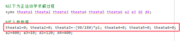
这是对应变量下的齐次变换矩阵 $_{6}^{0}\textrm{}T$ ：

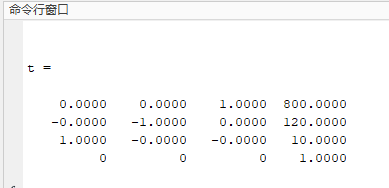
现在假设我们有了这个齐次变换矩阵 $_{6}^{0}\textrm{}T$ 的信息，我们把这个数据替换掉上面代码的a矩阵，然后运行程序：

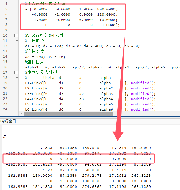
至此完成了逆运动学解算~

总结

本文以之前所写的正运动学《机器人正运动学实例——PUMA560机械臂（附Matlab机器人工具箱建模代码）》为基础，从基本公式推导出发，结合matlab工具完成了六自由度机器人的运动学逆解。最终能够实现输入指定的齐次变换矩阵，能够得到对应的所有变量解。这一过程有助于理解正逆运动学的分析过程，对于机器人设计及运动控制等有一定参考意义。

声明，本文的主要学习资料为 机器人运动学——林沛群老师课程

本文以学习为目的，会不断将所学总结更新，如有不足还望不吝赐教。