带你从入门到精通——知识图谱（四. 关系抽取）

最新推荐文章于 2025-06-13 16:51:50 发布

原创最新推荐文章于 2025-06-13 16:51:50 发布

· 977 阅读

27 ·

版权

文章标签：

#人工智能 #知识图谱 #关系抽取 #深度学习 #神经网络 #pytorch #pycharm

知识图谱专栏收录该内容

6 篇文章

订阅专栏

建议先阅读我知识图谱专栏中的前置博客，掌握一定的知识图谱前置知识后再阅读本文，链接如下：

知识图谱_梦想是成为算法高手的博客-优快云博客

4.4 BiLSTM with Attention模型

4.4.1 模型架构

4.4.2 模型示例

四. 关系抽取

4.1 关系抽取概述

关系抽取是指从给定的、包含两个及以上实体的文本中，预测实体之间的关系并抽取出关系三元组〈S，P，O〉，其中S表示subject，即主语、主实体、头实体，P表示predicate，即谓语、关系，O表示object，即宾语、客实体、尾实体，因此，关系抽取也属于文本分类任务。

关系抽取需要完成两大任务：首先是识别出文本中的实体对，其次是预测实体对直接的关系并抽取出关系三元组，正常来说关系三元组是没有重叠的，但是在某些情况下可能会出现SEO（Single Entity Overlap）问题或者EPO（Entity Pair Overlap）问题，SEO问题即单一实体重叠问题，该问题是指同一个实体参与到了多个关系中，EPO问题即实体对重叠问题，该问题是指同一个实体对参与到了多个关系中。

与实体抽取一样，常用的关系抽取方法可以分为基于规则和词典的关系抽取方法、基于传统机器学习的关系抽取方法以及基于深度学习的关系抽取方法三大类。

4.2 基于规则和词典的关系抽取方法

基于规则和词典的关系抽取方法主要是通过人工定义一些抽取关系的规则模式以及关系词典，从文本中抽取出关系三元组，示例如下：

import jieba.posseg as pseg

samples = ['李明是李雷的父亲', '王芳的妈妈叫张翠花',
           '周杰伦的弟弟是周杰明', '刘德华出演了无间道']
# 关系词典（使用字典直接映射）
rel_dict = {
    '父亲': '父子关系', '爸爸': '父子关系', '儿子': '父子关系',
    '母亲': '母女关系', '妈妈': '母女关系', '女儿': '母女关系',
    '哥哥': '兄弟关系', '弟弟': '兄弟关系', '兄弟': '兄弟关系'
}

if __name__ == '__main__':
    for sample in samples:
        people = []
        relation = None
        for word, label in pseg.cut(sample):
            if label == 'nr':   # nr表示人名
                people.append(word)
            if not relation:
                relation = rel_dict.get(word, None)
        print(f'原文：{sample}')
        if relation and len(people) >= 2:
            print(f'识别到实体关系对：{people[0]} -> {relation} -> {people[1]}')
        else:
            print('未识别到实体关系对')
        print('*' * 50)
    '''
    原文：李明是李雷的父亲
    识别到实体关系对：李明 -> 父子关系 -> 李雷
    **************************************************
    原文：王芳的妈妈叫张翠花
    识别到实体关系对：王芳 -> 母女关系 -> 张翠花
    **************************************************
    原文：周杰伦的弟弟是周杰明
    识别到实体关系对：周杰伦 -> 兄弟关系 -> 周杰明
    **************************************************
    原文：刘德华出演了无间道
    未识别到实体关系对
    **************************************************
    '''

基于规则和词典的关系抽取方法也有可移植性较差以及制作和维护成本太大的问题，而基于机器学习的关系抽取方法虽然增强了可移植性，但是仍然需要人工进行特征工程，有着较高的成本，下面主要介绍基于深度学习的关系抽取方法。

4.3 基于深度学习的关系抽取方法

基于深度学习的关系抽取方法主要可以分为两类，基于pipeline的关系抽取方法以及基于joint的关系抽取方法。

基于pipeline的关系抽取方法是指在已经完成实体抽取的基础上再进行实体之间的关系抽取，即先进行实体抽取，再将实体两两组合构成实体对，最后进行实体对之间的关系抽取，分步进行，这种方式的优点是实现了实体抽取和关系抽取的解耦，两者互不影响，但是pipeline方法无法处理EPO问题。

基于joint的关系抽取方法是指使用一个模型同时完成实体抽取和关系抽取，直接输出文本中包含的关系三元组。

4.4 BiLSTM with Attention模型

BiLSTM with Attention模型是用于实现基于pipeline的关系抽取的一种经典模型，

4.4.1 模型架构

BiLSTM with Attention模型结合了BiLSTM以及注意力机制，常用于处理文本分类任务，其模型的架构图如下：

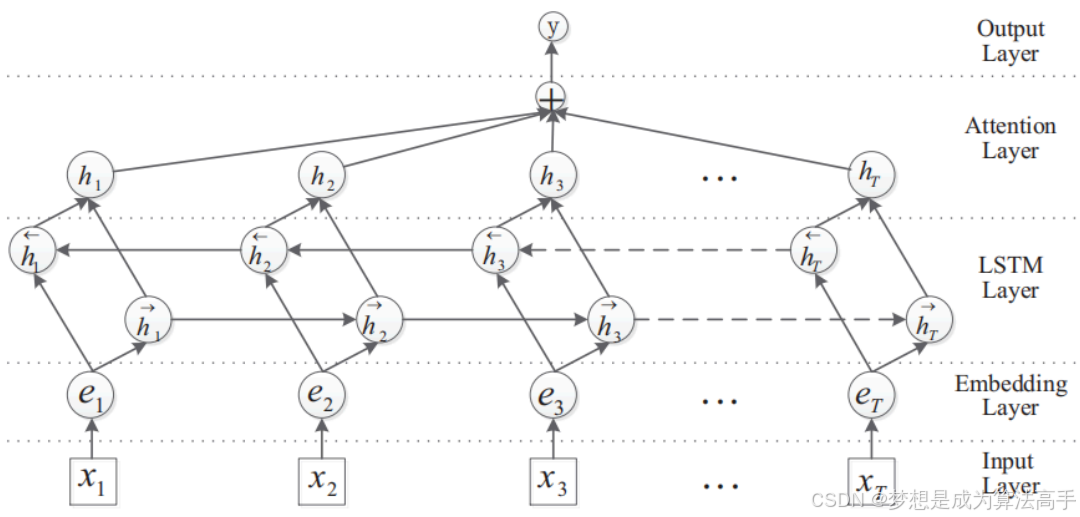
由上图可知，BiLSTM with Attention模型注意有五个部分：输入层、embedding层、BiLSTM层、Attention层以及输出层。

BiLSTM with Attention模型的训练数据需要有4个部分，即实体1、实体2、关系标签、原始文本。

BiLSTM with Attention模型的输入层需要接收三个输入，第一个输入为对原始文本进行label encoding后的形状为[batch_size，seq_len]的输入序列，第二个输入为输入序列的各个位置与实体1的相对位置编码序列，形状为[batch_size，seq_len]，编码方式是计算输入序列的各个位置与实体1的起始位置的差值，并且需要将差值映射到非负区间，第三个输入为输入序列的各个位置与实体2的相对位置编码序列，形状为[batch_size，seq_len]。

embedding层用于将三个输入序列分别映射为词向量后再进行concat拼接，输出一个形状为[batch_size，seq_len，text_embedding_size + position_embedding_size * 2]的张量。

BiLSTM层接收embedding层的输出张量，对其进行特征提取并输出一个形状为[batch_size，seq_len，hidden_size]的张量。

Attention层会在BiLSTM层的输出张量之间进行加性自注意力计算，对输出张量进行注意力重分配，最后在seq_len维度上进行求平均，得到形状为[batch_size，hidden_size]的上下文张量。

输出层则通过一个全连接层将Attention层输出的上下文张量映射成形状为[batch_size，label_size]的张量。

4.4.2 模型示例

BiLSTM with Attention模型的实现示例如下：

import torch
import torch.nn as nn
from relation_extract.utils.dataloader import getDataloader
from relation_extract.utils.preprocess import config, word2id, relation2id

class BiLSTMAttn(nn.Module):
    def __init__(self, config, vocab_size, label_size, pos_size):
        super(BiLSTMAttn, self).__init__()
        self.embedding_size = config.embedding_size
        self.hidden_size = config.hidden_size
        self.pe_size = config.pe_size
        self.batch_size = config.batch_size
        self.vocab_size = vocab_size
        self.label_size = label_size
        self.pos_size = pos_size

        self.word_embedding = nn.Embedding(self.vocab_size, self.embedding_size)
        self.pe1_embedding = nn.Embedding(self.pos_size, self.pe_size)
        self.pe2_embedding = nn.Embedding(self.pos_size, self.pe_size)
        self.lstm = nn.LSTM(self.embedding_size + self.pe_size * 2, self.hidden_size // 2,
                            batch_first=True, bidirectional=True)
        self.fc = nn.Linear(self.hidden_size, self.label_size)
        self.droupout_ebd = nn.Dropout(config.droupout)
        self.droupout_lstm = nn.Dropout(config.droupout)
        self.droupout_attn = nn.Dropout(config.droupout)

        self.Q = nn.Linear(self.hidden_size, self.hidden_size)
        self.K = nn.Linear(self.hidden_size, self.hidden_size)
        self.V = nn.Linear(self.hidden_size, 1)

    def attn(self, x):
        # q的shape为(batch_size, seq_len, 1, hidden_size)
        q = torch.unsqueeze(self.Q(x), dim=2)
        # k的shape为(batch_size, 1, seq_len, hidden_size)
        k = torch.unsqueeze(self.K(x), dim=1)
        # attn_score的shape为(batch_size, seq_len, seq_len, 1)
        attn_score = self.V(torch.tanh(q + k))
        # attn_score的shape为(batch_size, seq_len, seq_len)
        attn_score = torch.softmax(torch.squeeze(attn_score, dim=-1), dim=-1)
        # x的shape为(batch_size, seq_len, hidden_size)
        x = torch.mean(torch.bmm(attn_score, x), dim=1)
        return x

    def forward(self, x, pe1, pe2):
        x = self.word_embedding(x)
        pe1 = self.pe1_embedding(pe1)
        pe2 = self.pe2_embedding(pe2)
        x = torch.cat((x, pe1, pe2), dim=-1)
        x = self.droupout_ebd(x)
        x, (h, c) = self.lstm(x)
        x = self.droupout_lstm(x)
        # x的shape为(batch_size, seq_len, hidden_size)
        x = self.attn(x)
        # x的shape为(batch_size, hidden_size)
        x = torch.tanh(x)
        x = self.droupout_attn(x)
        # x的shape为(batch_size, label_size)
        x = self.fc(x)
        return x